Neural Networks
Table of Contents
- meta
- class notes
- 2010-08-24 Tue
- 2010-08-26 Thu
- 2010-08-31 Tue
- 2010-09-02 Thu
- 2010-09-07 Tue
- 2010-09-09 Thu
- 2010-09-21 Tue
- 2010-09-23 Thu
- 2010-09-28 Tue
- 2010-09-30 Thu
- 2010-10-05 Tue
- 2010-10-12 Tue
- 2010-10-19 Tue
- 2010-10-21 Thu
- 2010-10-26 Tue
- 2010-10-28 Thu
- 2010-11-02 Tue
- 2010-11-04 Thu
- 2010-11-16 Tue
- 2010-11-18 Thu
- 2010-11-23 Tue
- 2010-11-30 Tue
- 2010-12-02 Thu
- reading
- questions
meta
| Prof. | Thomas P. Caudell |
| Office | ECE Rm 235D |
| Text | "Neural Networks: a comprehensive foundation" Haykin Second Edition |
All homework should be submitted electronically
class notes
2010-08-24 Tue
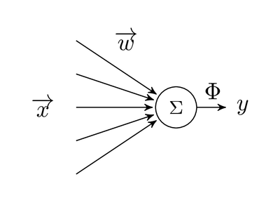
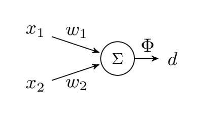
Canonical Model: embodied, always exist with inputs and outputs
- input vector \(\overrightarrow{x}\)
- many incoming axons with weights \(\overrightarrow{w}\)
- Σ of inputs \(v = \overrightarrow{w}^{T}\overrightarrow{x}\)
-
Φ some non-linear post-processing of sum
- pure linear identity
- binary on/off
- output y
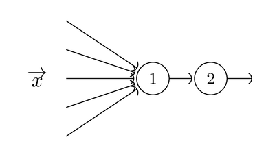
Structure
- single neuron
- levels of neurons
- trees of neurons
- arbitrary graphs (cycles) – this introduces time or memory into the system
2010-08-26 Thu
NN work initially derived from efforts to understand brain. Today we'll talk about biological models of the brain, basically all the stuff we'll be throwing out.
- neuron doctrine
-
brain composed of discrete cells, not one
contiguous tissue (emerged late 1800s)
0>----- 0>------ 0>------
two kinds of cells in the brain
- neurons
- 1010 neurons in the brain – many, many more at birth
- glial
-
~100 times as many glial as neurons
- interface between body and neurons blood brain interface
- clean up the waste produced by the neurons
- provide scaffolding/structure on which neurons grow
Three parts of neuron
    dendrites                   soma                  axons
    ---------                   ----                  -----
     inputs                   computer               outputs

 -----------\
             \            /------------------\
             |            |    soma          |
 ------------+            |    50nm          |  length 200microns -> 2m
             |            |                  |>-------------------------
             +------------+                  | \             ^
             |            |                  |  \            |
-------------+            \------------------/   \     myelin coating
             |                                    \
-------------/                                     axon hillock
general types of neurons
- unipolar
- dendrite and axon are connected to each other (no computing)
- bipolar
- dendritic tree and a single axon (as shown above) -- e.g. sensing, some dendrites in eye actually sense light, some in skin actually detect mechanical pressure, etc..
- multiple polar
- many bushy dendritic trees, and a single axon -- e.g. in spine and related to motor control
- pyramidal
- connical body with multiple potentially long dendritic trees out the point of the cone, and one branching axon coming out the base – in cerebral cortex, used for higher order cognition
- purkinje cell
- very well organized comb-like dendrites, can have 100s of thousands of inputs, used in motor control, in cerebellum
synapses
- electrolytes consisting of sodium, calcium, clourine, and potassium and ions (not electrons) which flow down axons as charge
- neurons have an internal negative charge on the order of 60-70 millivolts
- slowly accumulates positive charge until the axon hillock fires and send the charge down the axon and resets the neuron to a resting charge – this happens on a period of ~1ms
- pulse is regenerated on the way down the axon ensuring that the height and the width of the pulse is maintained from the beginning to the end of the axon – these are like voltage-dependent valves and pumps along the axon
- myelin, is mainly fat, so it looks white, so white matter in the brain is mainly connections, and grey matter in the brain has more neuronal bodies
- signals travel along an axon w/o myelin at ~10 meters per second, with glial cells wrapping the axon in myelin, which insulates portions of the axon s.t. those portions of skipped by the traveling spike resulting in clock speeds of up to ~100 meters per second
- max clock-speed of a neuron is ~1 kilo-hertz
- a typical neuron could have on the order of 10,000 synapses
reaction time
- for say breaking in your car can be ~ 1/2 second, that's like 5-10 serial steps of neurons, plus the flow down the spine to the motor control
synapse
                      /-----------------
                      |   Soma,
                cleft |   dendrite,
                ~30nm |   axon,
 ------------\        |   or even another
  synaptic   |        |   synaptic bulb
  bulb       |        |
             | chem   |
  transmits  | signal |
  electric   | -----> |
  sig to     |        |
  chem sig   |        |
 ------------/        |
                      |
                      |
                      \-----------------
learning takes place largely at the synapse, per electric pulse how much chemical is released.
2010-08-31 Tue
Input of charge along dendrites
- soma is constantly leaking charge
- each incoming impulse jumps up the charge in the soma
- inputs arriving at different distances down the dendrites will take different amounts of time to arrive
- complex spatio-temporal integration
Hebe's rules
-
if a neuron's fires are correlated with the firing of a synapse on
the neuron, then the strength of the synapse's effect on the neuron
will be increased
- (1) above is pre-synaptic neuron
- (2) above is post-synaptic neuron
- when they fire together the synapse increases in strength due to the sympathetic electrical and chemical processes
Cerebral Cortex flattens out to ~2sq feet ~imm thick, this is the darker gray matter (no myelin), under this sheet are bundles of connections between areas of the cortex (more mylin) white matter.
2010-09-02 Thu
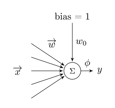
bias
in many cases learning can not take place without an initial bias,
where does this initial bias come from?
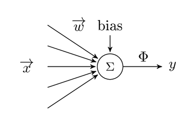 \begin{equation}
v = \Sigma^{n}_{i=1}w_{i}x_{i}+w_{0}
\end{equation}
bias can be considered (and implemented as) an axon with constant
input or a separate parameter to Σ
\begin{equation}
v = \Sigma^{n}_{i=1}w_{i}x_{i}+w_{0}
\end{equation}
bias can be considered (and implemented as) an axon with constant
input or a separate parameter to Σ
Π neuron
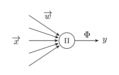 Unlike a Σ neuron, a Π takes the product of it's inputs rather than
the sum.
Unlike a Σ neuron, a Π takes the product of it's inputs rather than
the sum.
adapting activation functions (φ) weights and structures
(see reading-activation-functions)
activation functions (φ) in increasing complexity – these will all be monotonically non-decreasing (biological plausibility)
- constant
- linear
- piecewise linear
-
sigmoid \(\frac{1}{1+e^{-a(v+b)}}\)
- equals 1 at +∞
- equals 0 at -∞
- where a controls slope and b controls intersection at origin
- hyperbolic tangent, a sigmoid shifted down so it equals -1 at -∞
- there is one which is the most biologically plausible \begin{equation} \phi(v) = \frac{v^{2}}{1+v^{2}} \end{equation}
-
stochastic activation functions
- in one the neuron fires with some probability
- on the other type the output itself is a probability, however this is problematic because there is no way for a set of neurons to normalize their outputs, (probabilistic neural networks)
we like these to be
- monotonically non-decreasing
- bounded
- continuously differentiable
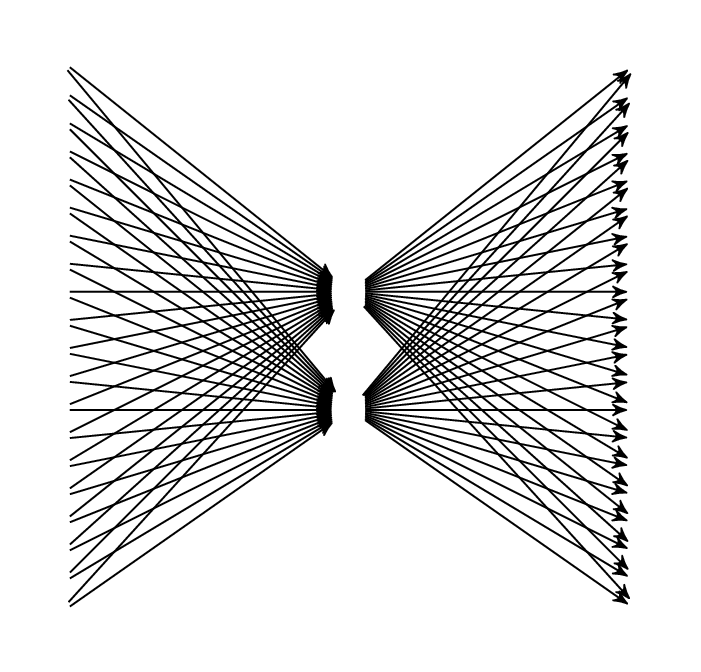
radial basis neurons
Rather than a sum or product of inputs, these take the difference between each input and its weight. So the larger the difference between the input vector \(\bar{x}\) and the weight vector \(\bar{w}\) the more active the neuron.
\begin{equation} v = |\bar{w}-\bar{x}|^{2} \end{equation}and \begin{equation} y = e^{-v^{2}} \end{equation}
architectures
layers
- input layer l0
- single layer has input and 1 processing layer (l1)
recurrent system
- like a single-layer feed forward, but all output neurons are connected (lateral recurrent system)
- or with outputs from some li going back into some lj s.t. j<i
recurrent systems can have very weird behavior, in terminology of control systems they are non-linear (see non-linear dynamical systems)
invariants
a variety of inputs can come from the same object (distance, orientation, etc…), needs to learn only this invariant information
2010-09-07 Tue
The text book is written by someone from a signal-processing background, he includes many flow-diagrams and we can ignore them if we like.
Today we'll finish Chapt. 1
- chapter 2 is learning
- chapter 3 is the first neural network chapter (single layer perceptron)
- chapter 4 multi-layer perceptrons
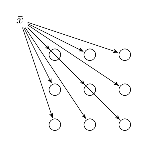
Structure
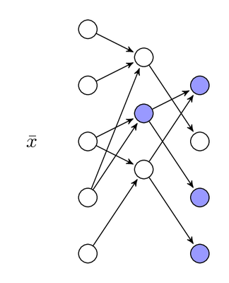
Activation (blue) of a network given an input $\bar{x}$
How do you represent knowledge in a neural network? Some pattern of activation in the network.
-
distance, ∀ \(\bar{x}\) ∃ some \(\bar{y}\) which is the activation
of the network due to the input. Each \(\bar{y}\) can be thought of
as a point in an n dimensional space (n neurons in the network).
We can take the Euclidean distance between these points as measures
of their similarities.
- Manhattan distance is L1 \begin{equation} L_1 = d_{kj} = |\bar{y}_{k} - \bar{y}_{j}| = \left(\sum^{n}_{l=1}{(y_{kl} - y_{lj})}^{2}\right)^{\frac{1}{2}} \end{equation}
- Euclidean distance is L2
- another interesting one is L∞
- also dot product of the vectors is interesting
- other metrics could be statistical, the mean of the activated values or something
-
edit or hamming distance
A metric or distance must be
- positive
- d \geq 0
- triangular
- d12+d23 \geq d13
- symmetric
- d12 = d21
- an important input should stimulate more neurons
- prior information can be built into the structure of the network or the pre-processor of the network
-
three ways to handle invariants – it's very possible for your
system to lock onto the wrong invariant if you're not careful in
selection of test data
- structure
- training
-
feature space transformation (preprocessing) e.g. we might
calculate the moments of each image in a series of images
- moments
-
the following are examples of moments, something
\(\frac{y(x)}{m_o}\) for input images could be used to control
for the overall brightness of the system, these can also be
used for translation (e.g. x'=(x-m1)), rotation,
etc… assuming there's only one item of interest in the
scene
- m0 = ∫∞ y(x) dx (area under the curve)
- m1 = ∫∞ y(x)x dx (expected value of x or mean)
- mn = ∫∞ y(x)xn dx
standard geometrical invariants
- translation – could add another layer that or's together a bunch of inputs from different locations
- rotation
- scale – ratios are invariant over different scales
2010-09-09 Thu
chapter 2
Consider a neuron w/2 inputs x1 and x2 and for each combination we have a desired output value d.
table of desired behavior
| x1 | x2 | d | y |
|---|---|---|---|
| … |
In this example let error e equal \(\frac{1}{2}e^2=(d-y)^2\), the \(\frac{1}{2}\) is there for the kinetic energy analogy.
Kinetic Energy \begin{equation} e = \frac{1}{2}mv^2 \end{equation} So for the above, lets make our neuron linear, and have our desired value be either positive or negative.
We want to minimize the error using a gradient descent algorithm. \begin{equation} w_1(n+1) = w_1(n)-\eta\frac{\delta e^2(n)}{\delta w_1} \end{equation} where η provides a scaling factor to convert between units of error and units of weight. So what's our derivative? \begin{equation} \frac{\delta e^2}{\delta w_1} = 2e()x_1() \end{equation}
- learning algorithms
- supervised vs. unsupervised
- local vs. global
- statistical vs. deterministic
- memorization vs. generalization
- fast vs. slow, meaning the rate of weight change per experience, fast learning typically involves allot of forgetting (see stability plasticity dilemma)
2010-09-21 Tue
on paper
2010-09-23 Thu
optimization
- ECE506 is entirely dedicated to optimization
we have some function, and we want to find the minimum

- we can do gradient descent with \begin{equation*} \bar{\Delta}E = \frac{\delta E}{\delta w_1}\hat{w_1} + \frac{\delta E}{w_2}\hat{w_2} + \frac{\delta E}{w_3}\hat{w_3} \end{equation*} to update our weights with \begin{equation*} \bar{w}(n+1) = \bar{w}(n) - \eta\bar{\Delta}E \end{equation*} Using this we can prove that the error will not increase. Considering the single-dimension case with a Taylor expansion \begin{eqnarray*} E(w(n+1)) &=& E(w(n))+\frac{\delta E}{\delta w} (w(n+1)-w(n) + \ldots\\ &=& E(w(n)) - \eta \left(\frac{\delta E}{\delta w}\frac{\delta E}{\delta w}\right) \end{eqnarray*}
- using Newton's Method we can compute the \(\Delta w\) required to take us directly to the minimum \begin{eqnarray*} \Delta E &=& E(w(n+1)) - E(w(n))\\ &=& \frac{\delta E}{\delta w}\Delta w + \frac{1}{2}\frac{\delta^2 E}{\delta w^2}\Delta w^2\\ &=& 0 \end{eqnarray*} so solving for \(\Delta E\) we can get \begin{eqnarray*} \Delta E &=& \frac{-\frac{\delta E}{\delta w}}{\frac{1}{2}\frac{\delta^2 E}{\delta w^2}}\\ &=& -H^{-1}(n)\Delta E(n) \end{eqnarray*} where H is a Hessian (and NxN matrix of all possible partial derivatives of a N-length vector)
training
we have a set of training vectors
| x | d |
for each training vector we can do gradient descent of the weights towards that vector
incremental learning
- linear φ \begin{equation*} w(n+1) = w(n) + \eta e(n) x(n) \end{equation*}
- non-linear φ \begin{equation*} w(n+1) = w(n) + \eta \phi'(v(n)) e(n) x(n) \end{equation*}
an epic is a run through all of our training vectors
after an epic we can assess our progress as the overall error \begin{equation*} E(k) = \sum_1^N{e^2(n)} \end{equation*} to get our cumulative error in the same scale as our per-vector error we can take the root mean square (RMS) error \begin{equation*} E_{RMS}(k) = \sqrt{\frac{1}{N}\sum_1^N{e^2(n)}} \end{equation*}
2010-09-28 Tue
Questions
- HW 2.12
- what is the question asking? these are two normalized Gaussians, we take the difference of these two Gaussians (Mexican hat). What happens if we translate this across along the x axis.
- HW 2.10
- two sums, write out the expression as the positive sum of the wx's minus the sum of the cy's or something… there are a number of ways this can be expressed
- general
- assume that the internal activation of a network under no input is set to 0
- Eulerian integration
- \(\frac{\delta y}{\delta t} = f(y)\), and we know the value at y=0. we can put this initial value in and use \(\frac{\delta y}{\delta t}\) to algebraically compute \(\delta y\) given some \(\delta t\). We can then just keep doing that.
Project
- this weekend we'll get the API code
- the first step is to run a dumb agent that does nothing or provides a random sequence of actions, we then try to beat that
-
so how could we use the LMS neuron for the project. we could use a
competitive layer of winner take all neurons along our line of
sight to select the brightest spot in our field of vision, then turn
towards that spot.
right before we eat an object we'll have a strong RGB input in our center neuron, we can treat this center neuron as an LMS neuron with a desired output of a positive \(\Delta energy\).
this could be a simple starting architecture.
- our experimental setup should report both average length of lifetimes and standard deviations on this length over a number of trials – maybe even a t test?
- if we want to we can exceed the page limit with an appendix of additional figures
- would be good to try to compute the upper bound on the possible life-span given some assumptions
- we'll get a tentative outline
Perceptrons
- error minimization
-
- linear φ
- minimize \(\frac{1}{2}e^{2}(n)\) where \(e(n) = d(n) - y(n)\)
- perceptron
-
- non-linear φ
- minimizing another criterion function aside from the squared error
2010-09-30 Thu
some current research uses complex numbers for activation propagation to propagate activation with a unit amplitude, but with both frequency and phase
perceptron
 with
\begin{equation*}
\phi = \left\{
\begin{array}{rl}
1 &: v > 0\\
-1 &: v \leq 0
\end{array}
\right.
\end{equation*}
the only other neural network architecture that provably converges is
adaptive resonance
with
\begin{equation*}
\phi = \left\{
\begin{array}{rl}
1 &: v > 0\\
-1 &: v \leq 0
\end{array}
\right.
\end{equation*}
the only other neural network architecture that provably converges is
adaptive resonance
2010-10-05 Tue
perceptron (cont)
- treat bias just like any other weight
- w0 is the bias weights, which is updated like any other
- if error then update weights with \begin{equation*} \bar{w}(n+1) = \bar{w}(n) + \eta(\bar{w}(old)-\bar{x}) \end{equation*} or \begin{equation*} \bar{w}(n+1) = \bar{w}(n) +- \eta\bar{x} \end{equation*} where if error means \begin{equation*} if \left\{ \begin{array}{rcl} \bar{w}^{T}\bar{x} \geq 0 &and& \bar{x} \in c_{+1}\\ \bar{w}^{T}\bar{x} < 0 &and& \bar{x} \in c_{-1} \end{array} \right. \end{equation*}
simulation of multilayer perceptrons
for a multilayer feed-forward network we can use a matrix representation of the neurons and their weights, then the running of the neural network could be reduced to matrix multiplication.
the following computes the activation \begin{equation*} \bar{v}(n+1) = \bar{W}(n) \bar{y}(n) \end{equation*} and the output of the entire network \begin{equation*} \bar{y}(n+1) = \Phi(\bar{v}(n+1)) \end{equation*}
multilayer perceptrons
- learning internal weights, how to update weights which are further back in the network?
2010-10-12 Tue
back-propagation learning
- dependencies
- E ← e ← y ← v ← w
- partial error
-
\begin{equation*} e_i = d_i - y_i \end{equation*}
- error
-
\begin{equation*} E(n) = \frac{1}{2}\Sigma_{i}{e^{2}_{i}(n)} \end{equation*}
- output layer
-
\begin{eqnarray*} \Delta w_{ij} &=& - \eta \frac{\delta E}{\delta w_{ij}}\\ &=& - \eta e_{i}\frac{\delta e}{\delta w_{ij}}\\ &=& - \eta e_{i} \frac{\delta e_{i}}{\delta y_{i}}\frac{\delta y_i}{\delta w_{ij}}\\ &=& \eta e_i \phi_{i}' y_i \end{eqnarray*} where \(\phi'_i = \frac{\delta}{\delta v_i}\phi_i(v_i)\)
- local gradient
- how the overall error changes as the activation of a single neuron changes \(\delta_{i}=-\frac{\delta E}{\delta v_i}\) and hence the change in weights between any two neurons is as follows \begin{equation*} \Delta w_{ij} = \eta \delta_i y_i \end{equation*} this is like local Hebbian learning
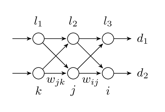
Now layer by layer
- Output Layer \begin{equation*} \Delta w_{ij} = - \eta \frac{\delta E}{\delta v_i} = \eta \delta_i y_i \end{equation*}
- Hidden Layer \begin{equation*} \Delta w_{jk} = - \eta \frac{\delta E}{\delta v_j}y_k \end{equation*} where \begin{equation*} \frac{\delta E}{\delta v_j} = \Sigma_i{e_i \frac{\delta e_i}{\delta v_j}} \end{equation*} and e changes with v, and y changes with v, and vi changes with vj… \begin{eqnarray*} \Delta w_{jk} &=& - \Sigma{e_i \phi'_i \frac{\delta v_i}{\delta y_i} \frac{\delta y_i}{\delta v_j}}\\ &=& - \Sigma{e_i \phi'_i w_{ij} \phi'_j}\\ &=& \eta y_k \phi'_j \Sigma{e_i \phi'_i w_{ij}}\\ &=& \eta \delta_j y_k \end{eqnarray*} finally we get \begin{equation*} \delta_j = \phi_{j}' \Sigma_i{\delta_i w_{ij}} \end{equation*}
Weight changes propagate back through the network, the δj is dependent on the sum of the δi's. The δ for each neuron need be computed only once.
This is a two-pass algorithm. for each pattern we pass through forward computing the v, y, and the φ' values, saving the y and φ' values. then on the way back we compute the e and φ' values to get the δ values of the output layer, and work backwards.
2010-10-19 Tue
note: there may be a mistake in the summary of back propagation section (eq. 4.47) the correct equation is (eq. 4.39)
back-propagation review
-
forward pass
- clamp on the inputs
- compute activations for nodes and their outputs through the network, and store these
- at the output we compute the errors ei(n)
-
backward pass
-
∀ layers
- compute the δ's, \(\delta_{j}(n) = \phi'_{j}\Sigma_{i}{\delta_{i}w_{ij}}\)
- compute the \(\Delta w(n) = -\eta \delta_{j}y_{k}\)
- calculate φ'
- loop back to the next previous layer and repeat
-
∀ layers
momentum
- without momentum \begin{equation*} \Delta w_{ij}(n) = - \eta \delta_{j}(n) y_{k}(n) \end{equation*}
- with momentum \begin{equation*} \Delta w_{ij}(n) = \alpha \Delta w_{jk}(n-1) - \eta \delta_{j}(n) y_{k}(n) \end{equation*} if α and -η sum to one, then the above is a convex combination
2010-10-21 Thu
Back Propagation Learning Algorithm
-
hidden neurons: compute and store on the forward pass
- \(v_j = \Sigma w_{jk}x_{k}\)
- \(y_{i}=\phi(v_{i})\)
- \(\phi'(v_{i})\)
-
output neurons: compute and store on the forward pass
- \(v_{i}= \Sigma w_{ij}y_{j}\)
- \(y_{i} = \phi(v_{i})\)
- \(\phi'(v_{i})\)
- then can compute the error as \(e_i = d_{i}-y_{i}\)
-
output neuron: backwards
- \(\delta_{i} = e_{i}\phi'(v_{i})\)
- \(\Delta w_{ij} = \eta \delta_{i} y_{j}\)
-
hidden neurons: backwards
- \(\delta_{j} = \phi'(v_{j}) \Sigma_{i}{\delta_{i}w_{ij}}\)
- \(\Delta w_{jk} = \eta \delta_{j} y_{k}\)
- finally do one more forward pass through the network in which we add all of the \(\Delta w\) values to our weights
For back propagation with momentum we save the old \(\Delta w\) so that we can use it to calculate our new \(\Delta w\). \begin{equation*} \Delta w_{ij}(n) = \alpha \Delta w_{ij}(n-1) + \eta \delta_{i} y_{j}(n) \end{equation*}
Training
- 2 inputs and 4 outputs
- for a full pass you can track a pattern error \(\frac{1}{2}\Sigma_{i}{e^{2}_{i}}\), however for a more intuitive metric it may be useful to look at the RMS error which is "of the same size" as the errors themselves \(\sqrt{\frac{1}{|i|}\Sigma_{i}{e^{2}_{i}}}\)
- the epic error could be taken as the RMS error over the entire set \(\sqrt{\frac{1}{|epic||i|}\Sigma_{n}\Sigma_{i}e_{i}^{2}(n)}\), we should plot these by epic
- after each epic we can turn off learning (backward pass) and compute the errors generated from the testing set of samples giving us another error (i.e. errortesting). We should plot both errortesting and errortraining on the same scale (note we should re-run the training data w/o learning). This is called a generalization plot.
- the training error will monotonically decrease, however it is possible that the testing error could begin to rise if we're over-fitting the training data.
- would be good to look at both incremental and batch update of the weights (e.g. do or do not update mid-epic)
- we should also look at how the order of presentation affects the performance of the network (only has an effect when doing incremental weight updates)
-
stopping criteria
- some error threshold
- testing error starts to increase
- etc…
- 3 architectures, 3 numbers of nodes, possibly to vary η, α, and even breaking some connections or removing some neurons after training to see how the network holds up
- weight initialization is yet another thing we could vary across multiple runs. There could be many local minima which we could land in depending on our starting position (or initial weights). For a given output neuron (expanded using a Taylor's expansion) \begin{eqnarray*} y_{0} &=& \phi\left[\Sigma_{i}w_{oi}[\Sigma w_{ij}x_{j}]\right]\\ &=& \Sigma_{l}a_{l}(\Sigma_{i}w_{oi}\Sigma_{m}a_{n}(\Sigma w_{ij} x_{i})^{m})^{l} \end{eqnarray*} So you could have a very large number of local minima. Typically you want to pick your weights in a random distribution centered around 0 – small weights lead to large values of φ' and large changes in weight.
2010-10-26 Tue
Bayes error is the theoretical best generalization error achievable. So for example in our back-prop assignment, we won't get better (at least on the test data) than the Bayes error which is around 13-14%. Note this is "classification error" or percent correct, not RMS error. This could be a good stopping criteria.
heuristics
(see convergence heuristics in the text book)
- you can look at the variance of your training data, and get a feel for what the σw of your weights should be
- for our homework assignment, the most effective solution will be to center our input data on the origin, and force a unit standard deviation on the input – this will keep us from saturating our neurons thereby reducing their information capacity to binary on/off. Note: this is a moment transformation, subtracting first moment and dividing by second moment.
- also, maybe set target values to something achievable (e.g. 0.1 and 0.9 instead of the asymptotic 0 and 1)
universal approximation theorem
(p.208 in the text)
For certain types of bounded functions over a finite domain ∃ a single-hidden-layer feed forward neural network which can arbitrarily approximate that function (i.e. ∀ ε ∃ a number n s.t. a network with n neurons in the hidden layer can approximate the function).
\begin{equation*} F(\bar{x}) = \Sigma_{i=1}^{n}\alpha_{j}\phi_{j}(\Sigma w_{ji}x_{i}+b_{i}) \end{equation*}This is like a Fourier Transform, a sum of orthonormal parts to approximate an arbitrary function.
back propagation to do other things
We could also for example take the partial of a (the slope of the sigma function) of a neuron, and use pack-propagation to adjust these values.
We can take partials of our inputs \(\Delta x_{i} = \eta \frac{\delta E}{\delta x_{i}}\) to guess what x would likely give us any particular output y. You would need an initial guess of inputs, but for any initial guess back-prop could be used to move form the guess input to another input which is more appropriate for a particular desired output.
2010-10-28 Thu
finishing off Chapter 4
- hidden layers can be used as feature detectors. if you force a large amount of data through a small hidden layer then the data will be compressed through that layer which will require discovery of structures in the data to achieve the compression. such hidden layers are sometimes called "feature detectors".
- Auto-associative network that maps inputs to identical outputs. This could also be used for compression or encryption. the bottleneck hidden layer could be considered a compressed (and probably unintuitive encryption) of the inputs.
- Introduce weight sharing where each neuron in the hidden layer shares the same weight structure (e.g. mexican hat). This could be used to for example build an apple detector over images, no matter where the apple is present in the original image the same weight pattern will be present near that part of the image.
-
prediction: say we have a time series, we can take a series of
values as input, and then take a single later value as the desired
output. In this way we can train a predictor.
              +--------+
 +----------->|   NN   |
 |            |        | output
 |  input     |        |--------+
 |       +--->|        |        |
 |       |    +--------+        |
 |       |                      |
 |       |                      v
-----------------------------------time-series-->
The "prediction company" formed out of the Santa Fe institute doing things like this for financial prediction.
-
In practice we won't know how to build a network, i.e. how many
layers and how many neurons in the layers. We want to limit the
complexity of the network. You can add a penalty term s.t. when a
weight has too much penalty it is removed.
- you can start big and cut things out, intermittently remove all small weights from the network, this won't remove neurons or layers but it will simplify the network
- you can add weights. start with a single neuron, doing learning with the standard Δ-rule. whenever an input results in a large error a new neuron is introduced which reduces that error and is connected to every existing neuron. The network is then trained through normal backwards propagation. These can work very well.
- GA, the chromosome is generally the adjacency matrix of the neural network (with a set number of neurons constant across the entire species). This matrix could be linearized out into one long vector. Then simple mutation and any length-preserving method of crossover can be used. More generally any method of graph crossover could be used.
radial basis neural networks
- φ-separability
- a data set is φ-separable if ∃ a function φ which separates the classes of the set
Covers Theorem: Any set of data with two classes (dichotomy) is more likely to be linearly separable the higher the dimension of the space in which the data is embedded.
as we non-linearly map our data into a higher dimensional space the linear separability of the data will increase. eventually we can just use a single perceptron to learn the data.
we can use radial basis neurons to perform this non-linear mapping
if we take a set of i functions φi, then we can use these i functions to map a point in 2 dimensions to a point in 2i dimensions by passing each coordinate through all i functions.
2010-11-02 Tue
Three smaller topics we'll be hitting
- radial basis neurons
- scalar vector machines
- committee machines
radial basis neurons
- H = {x1…xn}
- Dichotomy = (H1, H2)
- a set of functions \(\bar{\phi}(x)\)
a dichotomy is φ-separable if ∃ \(\bar{w}\) s.t.
- \(\bar{w}^{T}\bar{\phi}(x) > 0\) if \(\bar{x} \in H_1\)
- \(\bar{w}^{T}\bar{\phi}(x) \leq 0\) if \(\bar{x} \in H_2\)
radial basis network for X-or
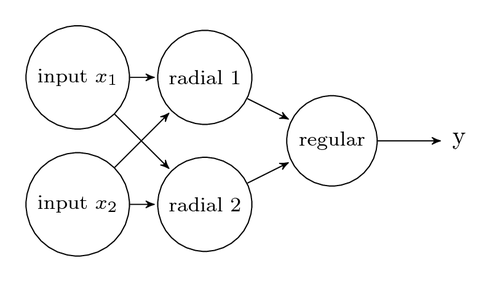
- \(\phi_1 = e^{-|x-t_{1}|^{2}}\) where \(t_1=(1,1)\)
- \(\phi_2 = e^{-|x-t_{2}|^{2}}\) where \(t_2=(0,0)\)
| x | φ1 | φ2 |
|---|---|---|
| 1,1 | 1.0 | 0.13 |
| 0,1 | 0.36 | 0.36 |
| 1,0 | 0.36 | 0.36 |
| 0,0 | 0.13 | 1.0 |
the non-linearly separable classes of Xor are mapped by φ1 and φ2 to a new plane in which they are separable
interpolative functions
An interpolative function will pass through all data points (even if it doesn't accurately reflect the behavior of the original function between the given data points).
F is interpolative if F(xi)=di ∀ i∈[1..N]
\begin{equation*} F(x) = \Sigma_1^{n}w_{i}\phi_{i}(x-x_{i}) \end{equation*}In matrix notation \(\Phi \bar{w} = \bar{d}\) or \begin{equation*} \left[ \begin{array}{ccc} \phi_{11} & \ldots & \phi_{1N}\\ \vdots & \ddots & \vdots\\ \phi_{N1} & \ldots & \phi_{NN} \end{array} \right] \left[ \begin{array}{c} w_{1}\\ \vdots\\ w_{N} \end{array} \right] = \left[ \begin{array}{c} d_{1}\\ \vdots\\ d_{N} \end{array} \right] \end{equation*} Then you can find the weight matrix in a single matrix inversion
A perceptron allows you to split a space with a hyperplane, however a radial basis neuron allows you to split a space with a hypersphere.
- Application
Let's say we want to fit a bunch of data with radial basis neurons using Gaussian functions for our φ's. If we have 10,000 data points and we only want 10 hidden neurons, then we could just pick 10 points at random to be the centers of our neurons. Random works very well because we tend to sample from dense sample areas.Since 10 does not equal 10,000 we can't use simple matrix inversion to learn our weights because a 10x10,000 matrix is not square.
we could also use
- clustering algorithms, or
- gradient descent – the free parameters in this approach above are the weights and the centers of the spheres, we could then computer the partial errors over δ-t and δ-w and descend on both the centers and weights
2010-11-04 Thu
learning on radial basis functions
(RBF learning strategies in the book p.320)
types
- random centers
- self organizing centers
- supervised – gradient descent centers
lets assume they're Gaussians for this example \begin{equation*} \phi(|\bar{x}-\bar{t}|) = exp(-\frac{|\bar{x}-\bar{t}|}{2\sigma^{-2}}) \end{equation*} So for a network with a hidden layer of m radial basis neurons all connected to all inputs and all feeding into a single perceptron the output is \begin{equation*} y=\Sigma_{i=0}^{m}w_{i}\phi(|\bar{x}-\bar{t_{i}}|) \end{equation*} initial values for our Gaussians
-
Under type (1) we set the centers ti to random input points, to
pick σ we want some overlap between the Gaussians positioned around
different centers, but we also want different values for points
closer to a particular center. So to approximate a good value for
σ we can find the maximum distance between any two pairs of
centers, and then we can set \(\sigma^{2} \simeq \frac{d_{max}^{2}}{\sqrt{m}}\).
Why do we divide this by \(\sqrt{m}\) (which is related to the dimensionality of the space)? Not sure, but this is an accepted heuristic.
Then to select the values for wi,
Once these initial values are selected we can use gradient descent to improve the values of wi ∀ i. The centers and the σ's are fixed, so we only need update the weights.
-
we select the centers using something like k-means. For k-means we
- pick a value of k (this is somewhat unsatisfying, we could start with only 1 center, and then add new centers whenever the max center to xi distance is over some preset threshold)
- randomly pick k centers (possibly from the data)
- loop over the data (xi's) and associate each x with the closest center
- for each center we move it towards the center of mass of the associated xi's by some learning parameter η
- keep doing it until the centers stop moving
- the standard deviations of these centers are easy to compute, just compute the standard deviation of the xi's assigned to each center
-
we can bring in a desired value, compute an error, and take the
partial errors along the weights, and then we can do gradient
descent on each of the hidden radial basis neurons.
If we think of every radial basis neuron as a function like \(\phi(\bar{x},\bar{t_{i}},\sigma_{i})\) then we can take partials of all three of the arguments to φ, e.g. \begin{equation*} t_{i}(new) = t_{i}(old) - \eta \frac{\delta e^{2}}{\delta \bar{t_{i}}} \end{equation*} We're still guessing at the number of hidden nodes, but having made that choice this works very well at moving around the centers of these nodes.
We can use a covariance matrix to allow σ to vary across dimensions, we could then learn these mi2 elements of the covariance matrix using gradient descent.
2010-11-16 Tue
last time
Hebbian learning in a winner take all system with a laterally connected output layer learning can be localized to the winner for any particular input.
self organizing maps
highly recommended book ← should purchase
| Title | Self Organization and Associative Memory |
| Author | T. Kohonen |
| ISBN | 3-540-18314-0 |
also this is Chapter 9 in the text.
The locations of neurons relative to each other in some space will begin to become important.
Imagine that all output neurons are embedded in a two dimensional planar grid. Imagine local inhibition of these output neurons on this 2D grid.
A self organizing map is a neural network which is continuous s.t. ∀ η ∃ δ s.t. if the output of two inputs x1 and x2 is within δ in the output space (our 2D plane) then x1 and x2 are within η in the input space.
typical representation of these 2D output neural networks
These neurons often have alternating competitive and cooperative phases. In normal competitive Hebbian learning only the winner has his weights changed, however in the Kohonen self-organizing map there is also a cooperative phase in which the winner shares learning with his neighbors, they share slightly less with their neighbors, etc…
- competitive
- first we find the winner by computing the cross product of the input \(\bar{x}\) with each weight vector \(\bar{w_{i}}\) and the winner is the neuron with the smallest inner product. \begin{equation*} J(\bar{x})=min_{j \in i,n}(||\bar{x} - \bar{w_{i}}||) \end{equation*} so the neuron with the weight vector closest to the x vector is the winner. We then move this weight vector slightly (by η) closer to the x vector.
- cooperative
-
For a generic neuron in the network
\begin{equation*}
\bar{w_{j}}(n+1) = \bar{w_{j}}(n) + \eta h(J(x))(\bar{x}(n) - \bar{w_{j}}(n))
\end{equation*}
where the \(h\) function need to return the highest values for
those neurons nearest to the winner with unity value right on the
winner and fairly quickly dropping to zero as we move away from
the winner. We can specify \(h\) as
\begin{equation*}
h(J(\bar{x}),j) = \left\{
\begin{array}{rl}
1 & j=J(\bar{x})\\
f(||\bar{r}_{J(\bar{x})} - \bar{r}_{j}||) & j \neq J(\bar{x})
\end{array}
\right.
\end{equation*}
or actually more like
\begin{equation*}
h(J,j) = exp\left(\frac{-d(J,j)^{2}}{2\sigma^{2}}\right)
\end{equation*}
where the distance metric
\begin{equation*}
d(J,j) = ||\bar{r}_{J} - \bar{r}_{j}||
\end{equation*}
and where σ is used to control the spread of the weight
propagation.
So how do you pick η and σ? At least initially you will want σ to allow the weight updates to touch most weights. Generally you will want to diminish both η and σ as time progresses.
pictured in the input space the following pretty much amounts to, whenever an input lands in the input space, all weights shift slightly towards that input with the degree of the weights movement based upon its closeness to the input (or rather its closeness to the closest weight).
There are some very cool demonstrations of and visualizations of these sorts of systems available on-line.
2010-11-18 Thu
continuous time systems – Hopfield network
we can turn our Canonical model into a continuous time differential equation, in which case we get \begin{equation*} \frac{\delta v_{i}(t)}{\delta t} = \Sigma_{i} w_{ij}(t) y_{i}(t) \end{equation*} This is similar to an RC circuit in which the input is the battery and the neuron is the capacitor.
Given this equilibrium equation… \begin{equation*} \frac{\delta v_{i}(t)}{\delta t} = \Sigma_{i} w_{ij}(t) y_{i}(t) - \frac{v_{i}(t)}{\tau} \end{equation*} When we first add input if the sum term is a positive constant, then the δ will initially be positive (because vi is initially 0), however eventually δ=0 when the sum equals the vi. This would be one time step in our model.
we also have… \begin{equation*} y_{i}(t) = \phi(v_{i},t) \end{equation*} these two equations together form a coupled system of non-linear equations.
some points
- if φ is linear then it is a coupled system of linear equations and would be more amenable to analysis
- there is no learning in the above, it gets considerably more complicated in this case \begin{equation*} \frac{\delta w_{ij}(t)}{\delta t} = F(?) - \frac{w_{ij}(t)}{\tau} \end{equation*} ultimately this is system of three highly related equations
- this system of equations can generally be bounded in space as the weights and activations won't normally go off to ∞
dynamical systems aside
- autonomous
- there is no explicit time term inside of the main function
- non-autonomous
- the function "F" does depend on time in some way e.g. \(F_{i}(\bar{x}(t),t)\)
because non-autonomous systems are very difficult we will focus on systems without an explicit time term.
so fixed points in the state space of this system of equations will correspond to states in which the neural network has ceased to learn and has learned some input, this can be thought of as a memory.
it is possible to linearize these differential equations in some bounded areas of space.
2010-11-23 Tue
after today we'll be doing adaptive resonance
basins of attraction
to study the stability of our "memory" attractors we'll be using Lyapunov's Theory (direct method) to determine if these attractors exist.
Lyapunov's Theory, assume ∃ V(x) which is
- continuous
- V(xstar)=0 where x^star is an attractor
- V(x)>0 when x ≠ xstar
In the range of the attractor (in its basin) \(\frac{\delta v(x)}{\delta t}<0\), this defines the region of the attractor (i.e. where \(\frac{\delta v(x)}{\delta t}<0\) is true).
neural dynamics
the application of dynamic systems analysis to neural networks
- additive model \begin{eqnarray*} \frac{\delta v_{j}(t)}{\delta t} = -v_{j}(t)+\Sigma_{i=1}^{n}w_{ji}(t)\phi(v_{j}(t))+I_{j}\\ y_{j}(t) = \phi(v_{j}(t)) \end{eqnarray*}
- alternate additive model \begin{equation*} \frac{\delta y_{j}(t)}{\delta t} = -y_{j}(t)+\phi(\Sigma_{i=1}^{n} w_{ij}y_{i}) \end{equation*}
Hopfield Network and Stability
with
- wji = - wij
- the φ function is invertible
- and ∃ a Lyapunov's function \begin{equation*} - v = - \frac{1}{2} \Sigma_{i=1}^{n} \Sigma_{j=1}^{n} w_{ji}y_{j}y_{i}+ ORG-LIST-END \Sigma_{j=1}^{n}\frac{1}{\tau}\int_{0}^{y}\phi^{-1}_{j}(y)\delta y - \Sigma_{j=1}^{n}I_{j}y_{j} \end{equation*}
- \(\frac{\delta v}{\delta t} < 0\)
2010-11-30 Tue
Adaptive Resonance Theory ART-1
               +--------------------+      dipole layer, each neuron is a pair
F2             |o o o o o o o o o o |   <- connected as a flip-flop, and all
               +--------------------+      pairs connected as winner-take-all

                                               +----+   gain control
             Full Bidirectional connectivity   | GC |<- fully connected
              (top down weights are binary)    +----+   to F1 and F2

    +---------------------------------------------+
F1  |o o o o o o o o o o o o o o o o o o o o o o o|
    +---------------------------------------------+    +---+    vigilance,
      ^        ^    ^           ^      ^     ^         | e | <- fully connected
      |        |    |           |      |     |         +---+    to F1 and F0
    +---------------------------------------------+
F0  |o o o o o o o o o o o o o o o o o o o o o o o|
    +---------------------------------------------+
       ^         ^       ^       ^           ^
       |         |       |       |           |

           Input I is binary vector
Neurons
- GC
- is on unless it is inhibited, any inputs turn it off
- F0
- these neurons are binary on or off depending on their input
- F1
- these are threshold neurons, which have three inputs (one from F0, one from GC and one from each neuron in F2 which is initially only 1), it requires at least 2 inputs to turn on
- F2
- each neuron is a flip-flop pair of neurons with the whole layer connected into a winner-take all network, let Ti be the weights up from F1 to neuron i in F2, then the downward weights of i Bi are always a binary scaling of Ti
- e
- the vigilance neuron checks the Hamming distance between the activation of F0 and the activation of F1, to see if the top-down weights (defining the center of the active neuron in F2) is close enough to the input (the activation in F1), we can calculate this with \begin{equation*} \frac{||T_{1}-I||}{||I||} \geq \rho \end{equation*} where T1 is the activation pattern of F1 and I is the input vector. e turns on when the activation is less than ρ. When e turns on it activates the flip-flop neuron of the active neuron in F2 which latches off F2, and when the effects of F2 turning off propagates through the network and the original input activation propagates back up to F2, a new neuron is recruited to activate in response to the input.
Lets look at the behavior of this system
- initially only GC is turned on
- lets apply a pattern
- the F0 neurons of the 1 inputs will activate
- the F1 neurons related to the active F0 neurons will activate (because they now have two inputs)
- the active F1 neurons then push activation to the recruited neurons in F2, and the winner turns on
- when the winner turns on it begins activating GC and activating back from F2 to F1 (according to its top-down weight vector)
- without GC on all neurons in F1 which aren't activated by the active neuron in F2 turn off, those neurons in F1 which are turned on are now the intersection of those in the input pattern and those with top-down weights from the active neuron in F2
This is like leader clustering where we test for closest and close-enough. The closest part of this is controlled by the winner-take-all formation in F2, the Vigilance neuron e is responsible for the close-enough test.
We then learn the weights between F1 and F2 with Hebbian learning. All weights are held between 1 and 0, as the activation resonates then those neurons in F1 which resonate with the active neuron in F2 will have their weights to and from F2 tend to 1 and all others have their weights tend to 0. This is similar to template matching in the pattern matching literature.
2010-12-02 Thu
Adaptive Resonance Theory ART (continued)
           k=1             nf2
     +---------------------------+
   F2|     ------------------    | \
     |                           |  |
     |        T                  |  |
     |         k                 |  |
     |                           |  |
   F1|  -----------------------  |  |
     |                           |\ /
     |                           | e
   F0|  -----------------------  |/
     |                           |
     +---------------------------+
- closest
-
How do we compute the closest neuron in F2?
The activation normalized by the number of up weights (size of the template) \begin{equation*} k = argmax_{k=1,nf2}\left\{\frac{||I \wedge T_{k}||}{\beta + ||T_{k}||}\right\} \end{equation*} β has the effect of breaking ties in favor of the larger template, β is typically set to \(\frac{1}{nf0}\).
- close enough
-
How do we decide if this is close enough
\begin{equation*} \frac{||I \wedge T_{k}||}{||I||} \ge \rho \end{equation*} If the above is not true, then we reset and add a new neuron to F2
If it is true then we learn and update Tk using the gated Hebbian we discussed last time
↑ the above is the entirety of the ART algorithm ↑
some properties:
- this can all be described by a set of coupled differential equations
- the order of presentation of training points affects the learned structure
limits on the maximum required number of epics
we can prove this using compliment coding – meaning ∀ inputs I we concatenate I and its compliment IC (I,IC). The size of this concatenation will always be equal to the number of bits in I.
This will converge (number of nodes and values of weights) in 1 epic.
how to use real-valued inputs
thermometer code
- normalize your inputs to between zero and 1
- then multiply each normalize value by nf0 and represent it by that many consecutive 1's and pad the rest with zeros
this real value case with unary encoding can be very easily visualized geometrically where every neuron in F2 becomes a box in the number of dimensions as there are real values in the input
fuzzy-ART
- we replace ∧ with a fuzzy-∧ which is just min, it returns the min of its inputs (which don't have to be 0 or 1 but can be any real value between 0 and 1).
- similarly compliment becomes 1- so the compliment of (0.1,0.3) becomes (0.9,0.7)
ART-2
Not very popular, is the case where the F2 row is not winner-take-all but rather can have multiple neurons turn on.
ART-Map
for supervised learning
                   x
                  / \
                 /   \
                x     x Association Matrix
                 \   /
                  \ /
                   X


    +----------+      +----------+
    |          |      |          |
    |    A     |      |    B     |
    |          |      |          |
    |          |      |          |
    +----------+      +----------+
        x                  d
x and d are the inputs and the desired values, these train A and B which are both ART-1 architectures, and their outputs go into an association matrix in which the related outputs are associated.
reading
1st Chapter
Benefits of Neural Networks
- nonlinearity
- in the weighting between neurons, each neuron is non-linear as are their sum
- input-output mapping
- ideal for supervised learning
- adaptable
- easily re-weighted to adapt to a changing environment, however shouldn't change to fast to fleeting disturbance this is called the stability-plasticity dilemma
- evidential response
- can return confidence along with it's clarifications
- contextual information
- each neuron can potentially affect each other neuron allowing for natural spread of contextual information
- fault tolerant
- naturally distributed so if any single neuron is damaged the global behavior is not impaired but not drastically affected robust, graceful degradation
- VLSI
- massively parallel, take advantage of parallel hardware
- uniform
- regardless of problem domain the same structure (interconnected neurons) is used, allows for modularity and composability
- biological analogy
- as an analog of a biological system, many good ideas can be borrowed from nature
Types of activation functions
(see notes-activation-functions)
- Threshold
-
\begin{equation} \phi(v) = \left\{ \begin{array}{lcl} 1 &if& v \geq 0\\ 0 &if& v < 0 \end{array} \right. \end{equation}
- Piecewise Linear
-
\begin{equation} \phi(v) = \left\{ \begin{array}{lcl} 1 &if& v \geq +\frac{1}{2}\\ v &if& +\frac{1}{2} > v > -\frac{1}{2}\\ 0 &if& v \leq -\frac{1}{2} \end{array} \right. \end{equation}
- Sigmoid
-
\begin{equation} \phi(v) = \frac{1}{1+exp(-av)} \end{equation}
- Stochastic
-
\begin{equation} \phi(v) = \left\{ \begin{array}{lcl} +1 &\text{with probability}& P(v)\\ -1 &\text{with probability}& 1-P(v) \end{array} \right. \end{equation} where \begin{equation} \phi(v) = \frac{1}{1+exp(-v/\tau)} \end{equation} where τ is a pseudo temperature used to control the amount of noise in the system
Network Architectures
- single-layer feed-forward
- single layer of input nodes which connect to a single layer of output nodes, acyclic
- multi-layer feed-forward
- like the above but with hidden layers between the input and output layer, these can be particularly useful when the size of the input layer is large. These are fully connected when every node on a layer is connected to every node on the adjacent layers
- recurrent networks
- neural networks which has as least one feedback loop, which will typically involve unit-delay elements. feedback loops have significant effect on the behavior of the network
Knowledge Representation
It is difficult to talk about knowledge being represented inside of a neural network, as any such knowledge will be stored implicitly in the structure of the network. As such any knowledge which a neural network may contain about it's world (inputs and outputs) is directed toward acting in the world.
Knowledge Rules
- similar inputs from similar outputs should result in similar (e.g. by Euclidean distance of a vector of neuron activation) internal states and should thus be classified similarly
- opposite of (1) items in different categories should be given different internal representations
- important features should be allotted a large number of neurons in the network
-
prior information and invariance should be built into the design of
the network
- biologically plausible
-
smaller size
- limits the search space of the network
- faster information transition through the network
- cheaper to build becu
How to Build Prior Information and Invariance into a Network
no general rules.
two ad-hoc rules for prior information
- Restricting network architecture through use of local connections known as receptive fields
- Constraining the choice of weights through weight-sharing
invariance, e.g. same object but viewed form different angles, same voice but spoken loudly or softly
methods of entraining invariance into a network
- invariance by structure
- invariance by training
- invariant feature space, assuming ∃ features which are constant across all variants of the same input
2nd Chapter
Learning
- neural network is stimulated
- it changes
- it responds differently because of the change
learning paradigms
- Error-correction Learning
- directed to a particular neuron
- the output of that neuron is compared to the desired output
- the difference error is used to re-weight the inputs to the neuron
- this process continues until the neural net hits some steady state
(this is implemented with back-propagation)
- Memory-based Learning
- each input is associated with an output
- when a new unknown input is seen it is classified as the same value as the nearest (Euclidean) known input
- Hebbian Learning
associative learning- if the neurons on either side of an axon are activated simultaneously then the strength of the axon is increased
- if the neurons are activated asynchronously then the synapse is weakened or eliminated
this sort of learning is
- time-dependent
- local
- interactive (depends on both side of the synapse)
- conjunctional or correlational
strong physiological evidence that associative Hebbian learning takes place in the brain
- Competitive Learning
- each input neuron is attached to every output neuron
- random weights on all of these attachments
- for each set of inputs the output neuron with the highest activation is the winner, and all of it's active input connections are strengthened
- this process continues until the weights stabilize
with k output neurons this performs similar to k-means clustering, in which each output neuron is finally associated with a cluster of similar inputs
- Boltzman Learning
the neural network or Boltzman machine is characterized by an energy function. \begin{equation} E = -\frac{1}{2}\Sigma_{j}\Sigma_{k \neq j}w_{kj}x_{k}x_{j} \end{equation} the machine operates by selecting a neuron at random during the learning process and flipping it's output with probability \begin{equation} P(x_{k} \rightarrow -x_{k}) = \frac{1}{1 + exp(-\Delta E_{k}/\tau)} \end{equation} two running conditions- clamped condition in which the visible neurons (attached to the environment) can't be changed
- free-running condition in which all neurons can be flipped
let
- \(p_{kj}^{+}\) denote the correlation between neurons j and k when in clamped condition
- \(p_{kj}^{-}\) denote the correlation j and k when free-running condition
then the change in weight is \begin{equation} \Delta w_{jk} = \eta(p_{kj}^{+} - p_{kj}^{-}), j \neq k \end{equation}
credit assignment problem
how to assign credit and blame to inner portions of a neural network, this is sometimes complicated through temporal delay, requiring assignment of credit to past actions/events
Learning without a Teacher
these first two require a critic
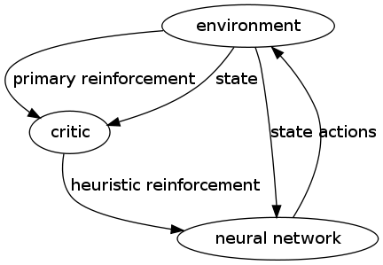
Reinforcement Learning with a critic
- in reinforcement learning the system matches input to output to maximize some scalar performance measure.
- in delayed reinforcement learning the system attempts to minimize a cost-to-go function, which is the cost of a sequence of actions taken over some sequence of inputs. learn from the results of actions. related to dynamic programming
Unsupervised learning w/o a critic
an example of unsupervised learning: a two-layer neural network in which the first layer is the input layer and the second the competitive layer, s.t. the neurons in the competitive layer compete with each other to respond to an input.
learning tasks
- pattern association
- associative memory
- distributed memory which learns by association
- auto-association
- (unsupervised) a set of patterns are repeatedly presented to the network, and it tries to store them s.t. when presented with a noisy version of a pattern it returns the original pattern
- hetero-association
- (supervised) arbitrary set of input patterns are paired with another arbitrary set of output patterns
- pattern recognition
assignments of inputs to classes
classical design for pattern association network
- function approximation
Attempt to match some function \(d = f(x)\) where x is the input vector and d is the desired output. Supervised learning can be used to train the network to match \(f\).
questions
- in implementations, is a neuron normally allowed to reference itself?
- what state is normally contained in a neuron?