Comprehensive Exam Preparation
Table of Contents
Topics
OS
threads – dinosaur 4
(see threads)
scheduling – dinosaur 5
(see scheduling, proportional share scheduling, lottery reading, lottery scheduling)
run multiple process on a single CPU with the goals of
- mimicking a multi-cpu environment
- maximally utilizing the cpu e.g. while one process is I/O blocking let other processes run
The average length of time processes run the cpu between I/O interrupts can be important for the selection of a scheduler
Scheduling decisions can be required in response to the following four conditions
- process switches from the running state to the waiting state (e.g. due to I/O request)
- process switches from running to ready (e.g. due to interrupt)
- process switches from waiting to ready (e.g. I/O completes)
- process terminates
in nonpreemtive or cooperative scheduling, processes are only swapped in cases (1) and (4) above, otherwise the scheduler is preemptive
the dispatcher is responsible for
- switching context
- switching to user mode
- jumping to the proper location in the user program to restart the program
scheduling criteria
- cpu utilization
- want to keep the cpu running all the time
- throughput
- number of processes completed per unit time
- turnaround time
- interval form time of submission to time of completion
- waiting time
- sum of the amount of time spent waiting i the ready queue
- response time
- time from submission to first response
- scheduling algorithms
- first-come first-serve
-
easily managed and programmed with a FIFO
queue
average wait time is often very long – e.g. when a long-running process is the "first in"
not good with cpu maximization, say ∃ one cpu bound process and many i/o bound processes – the scheduler will continually cycle the FIFO queue, whenever the cpu bound process gets the cpu, then the i/o all completes, and all i/o devices and processes sit idle while the cpu process churns, after it finished all the i/o processes cycle in a quick succession of tiny bursts, and we're back to the beginning with most resources and processes idling. this is called the convoy effect.
- shortest job first
-
associated with each process is the length of
it's next cpu burst – always run the shortest job first.
provably optimal for minimum average waiting time
impossible to know the length of a processes cpu burst before hand – generally this is estimated to be the exponential average of a processes recent cpu burst lengths
- priority scheduling
-
a priority is associated with each process,
and the cpu is allocated to the process with the highest priority
(in SJF above the priority is based on expected wait time).
indefinite blocking or starvation, low-priority jobs may never get on the cpu
rumor has it that, when they shut down an IBM 7094 at MIT in 1973, they found a low-priority process that had been submitted in 1976 and had not yet been run
a solution to this problem is aging. aging gradually increases the priority of a process with it's time since last cpu burst
- round robin
-
designed specifically for time-sharing systems.
similar to FCFS with preemption, a time-quantum or time-slice
(generally 10-100 milliseconds) size is defined, the queue is
treated as circular, and the cpu scheduler going around the queue
doling out time slices.
with very large slices RR ≅ FCFS
with very small slices 1 cpu and n processes looks like n cpu's working at 1/n speed (less context switching time)
context-switch-time/slice-time = % time spent context switching
- multilevel queue scheduling
-
different classes of processes,
e.g. foreground (interactive) and background (batch) process
partitions the ready into many different queues. processes are permanently assign to one queue. each of which can have it's own algorithm (e.g. RR for interactive, FCFS for batch).
inter-queue scheduling is generally handled with something like a fixed-priority scheduler (e.g. foreground before background)
- multilevel feedback queue scheduling
-
like the above only it is
possible for processes to switch queues. the idea being to
assign processes to queues based on their cpu burstiness.
for example say ∃ 3 queues of increasing time quanta. a new process is added to the top (fastest) queue. if it doesn't complete in it's time quanta, then it's demoted to the next queue.
parameters
- number of queues
- scheduling algorithm for each queue
- method used to determine when to upgrade a process to a higher queue
- method used to downgrade a process
- method used to place newly arrived processes into an initial queue
- multi-processor scheduling
- in asymmetric multiprocessing one cpu handles all scheduling decisions and all other cpus only run user code – this reduces the need for sharing system data among cpus.
- in symmetric multiprocessing each processor is self-scheduling, all processes may be organized in a common ready queue, or each processor may have it's own ready queue.
generally it's preferable not to switch a process from one cpu to another for things like cache memory – the inclination to keep a process on it's most recent cpu is called processor affinity
load balancing is important to take advantage of the all processors. a common queue makes load-balancing unnecessary, but is generally not desirable. Two approaches to load balancing are push migration and pull migration
- push migration
- a specific task checks the load on each processors and potentially distributes the load by migrating processes
- pull migration
- idle processors pull tasks from loaded processors
there is a tension between processor affinity and load balancing
synchronization – dinosaur 6
coordination of light weight processes
a solution to the problem of competing critical sections must satisfy the following three requirements
- mutual exclusion
- If process Pi is executing its critical section then no other process can be executing in their critical section
- Progress
- if critical section is open, and some processes want to enter their critical section then only those processes not in their remainder section can participate in the decision, and the decision must be reached in finite time
- Bounded waiting
- ∃ a bound on the number of times other processes are allowed to enter their critical sections while ∃ a process waiting to enter its own critical section
the OS is fertile ground for race conditions
- non-preemptive kernels
- protect against race conditions by never interrupting a process in it's critical secton
- preemptive kernels
- more complicated because it requires synchronization of shared kernel data, but better for real time performance and protection against arbitrarily long running critical sections
hardware support in the form of instructions for atomic
test-and-modify (e.g. TestAndSet()) behavior or word-swapping
behavior
-
with
TestAndSetwhile(TestAndSetLock(&lock)) ; // do nothing
-
with
Swapkey = true; while(key == true) Swap(&lock, &key);
-
an integer variable which (apart from initialization)
is only accessed through two methods
-
wait()ortest()wait(s) { while(s <= 0) ; s--; }
-
signal()orincrement()signal(s) { s++; }
the values of counting semaphores can have an arbitrary range, while binary semaphores (or mutexes see monitors) can only have the value of 0 or 1. The initialized value of the semaphore determines how many process can concurrently use the resource
-
the main downside to semaphores is that they require busy waiting or spinlocks where a process burns cpu while waiting on a resource. this can be overcome with a wait queue, and processes which block when a resource is busy and then wait on the queue until the receive a "wakeup" signal.
-
semaphore with a wait queue
typedef struct {
  int value;
  struct process *list;
}
-
wait()wait(semaphore *s){ s->value--; if (s->value < 0){ add_self_to_queue(s->list); block(); } }
-
signal()signal(semaphore *s){ s->value++; if(s->value <=0){ p = remove_from_queue(s->list); wakeup(p); } }
note that these wait() and signal() operations are themselves
critical sections, and are generally guarded by a simple lock like a
spin lock.
- monitor
-
high-level programming language construct used to provide
safe programmer-error free use of semaphores and mutexes
programmers define variable declarations and critical operations inside the monitor, and then the monitor provides synchronization protection for those variables and methods
monitor{
  // shared variable declarations
  procedure p1(...){
  }
  procedure p1(...){
  }
  // ...
  initialization(){
  }
}
for custom synchronization needs not addressed by the predefined methods monitors may also expose condition variables (e.g.
x) which can providex.wait()andx.signal()operations which are like their semaphore alternatives but are safer.in general monitors can be misused in the same way as semaphores
- atomic transactions
-
a series of
readandwritecommands terminated by either acommitor anabortcommit- the effect of the previous reads and writes are applied to the system
abort- all previous actions are rolled back
one solution to providing these features is write-ahead loggin in which each action is logged before it is propagated to the system. in these systems the entire state can be recreated by re-running the log, however each logical write requires two physical writes, and the logs take up as much space as the actual data.
When restoring data, any transaction with a <Ti starts> and no <Ti commits> need not be applied to the database.
we can use checkpoints to increase the efficiency of rebuilding our data. the system will periodically execute a checkpoint which involves
- output all log records currently residing in volatile storage (e.g. memory) to disk
- output all modified data to disk
-
output a log record
<checkpoint>onto stable storage
when multiple transactions are active simultaneously the execution of the transactions must be equivalent to the case where these transactions are executed serially in some order -- this is called serializability
if a schedule can be transformed into a serial schedule by a series of swaps of nonconflicting operations we say that it is conflict serializable
a single transaction may require locks on a number of data objects, to ensure serializability the sequence of locking and unlocking should happen in two phases
- a growing phase in which the transaction can acquire but not release locks
- a shrinking phase in which the transaction can release but not acquire locks
alternately a time-stamp based approach can be used to implement serializability, in which each item is associated with both a
- read-time-stamp recording the time of the last successful read, and a
- write-time-stamp recording the time of the last successful write
these can be used to organize any conflicting operations into a single conflict-free series.
memory – dinosaur 8
- memory layout and compile times
- base register
- smallest legal address
- limit register
- largest legal address
addressing spaces
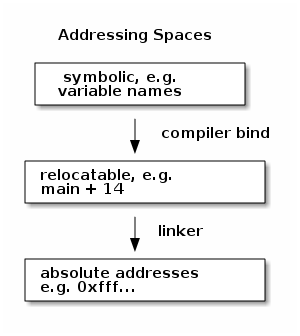
bound at
- compile time
- if you know where program is to run in memory
- load time
- compiler makes relocatable code → bound at load time
- exec. time
- lets process move during execution, requires special hardware
- MMU
-
converts logical (virtual) addresses into physical addresses,
this enables the exec. time binding mentioned above
the base register is used as an offset register, it is added to every address
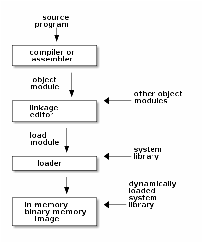
- dynamic loading
-
each routine is loaded as needed, so…
- many parts of the program may never need to be brought into memory
- system libraries can be shared between processes (with some OS help at link time)
- stubs
- placed in executables where system libraries would go, they handle checking if the needed routine is in memory (with OS help), and then if they load it into memory then they replace themselves with a jump to the address of the system routine in memory
- swapping
-
moving processes between main memory and the backing
store
if compile or load time binding, then the process must always be swapped into the same part of main memory
for efficiency in multiprogramming environments you always want the time quanta to be greater than the swap time
if a swap is needed for a process waiting for I/O you must either let the I/O complete, or handle all I/O to/from OS buffers, so that processes don't overwrite each other's address spaces with stale I/O.
- memory allocation
how to break up main memory- fixed size partitions
-
1 big hole which is filled with…
- first fit
- each proc takes the first big enough space
- best fit
- each proc takes the space closest to it's requirements
- worst fit
- always put in the biggest space – because biggest remainder
non-contiguous memory
- paging
-
segmentation
logical memory physical memory frames pages - paging
a standard size is used for memory allocationhigh order low order bit bit | | v v address \rightarrow [page #, page offset] | +---------- | page table | memory | +----+ | | | | | | index +----+ physical offset | +--------------> | | ------------------> | +----+ | | | | +----+ | | | | +----+ | +----------- 1 page table per process
-
stored in
- dedicated registers – fast but small
- page table base register points to table in memory, slow
- TLB – small, fast, associative hardware cache, when accessed compares against all keys simultaneously, can only hold part of the page table sometimes you'll get a TLB miss and have to go to memory
-
ASID – Address Space ID
- relates processes to address spaces
- means that the TLB need not be flushed between processes, just entry by entry as the spaces fill up
- protection
bits w/each page-table entry can specify read-only or read-write, execute-only, and more importantly- valid/invalid bit
- protect non-user/process accessible pages in the page table
paging allows for shared pages say everyone uses Emacs, only one Emacs in memory
- structure of page table
- hierarchical paging
-
multi-level page tables, further divide page number
 page number | offset
+---------------------+
|  p1 |  p2  |        |
+---------------------+
up to 4 levels of page tables on some 32-bit machines, generally not deemed appropriate for 64-bit machines
- hashed page tables
- page number is a hash key, page table is a linked list of [hash key, page address, offset] elements, in clustered page tables each key points to 16 pages rather than just 1
- inverted page table
- table is indexed by actual memory addresses, and each element holds the related virtual addresses, this decreases the size of the page table, but increases the time required to use it as processes must search through the table to find the entry for their virtual address
- segmentation
a logical address space is a collection of variable length named segments each of which has a name and a length<segment number, offset>
these are mapped through a segment table to turn the segment number and offset into memory addresses
  segment table
   +-----+----+
   |     |    |
   |limit|base|
   |     |    |
   +-----+----+
can be used with paging
          logical            linear            physical
           addr               addr              addr
 +------+       +-----------+      +-----------+      +-----------+
 | CPU  |------>|sementation|----->|  paging   |----->| physical  |
 |      |       |   unit    |      |   unit    |      |  memory   |
 +------+       +-----------+      +-----------+      +-----------+
virtual memory – dinosaur 9
- executing code must be located in physical memory, although rarely is the entirety of a program needed for it's execution – parts handling edge cases, variables that never reach their full potential size, etc…
- virtual memory allows programs to address virtual memory which could be much larger than physical memory, the process references it's memory through a virtual address space which the OS maps to physical memory
- sharing and virtual memory
- for system libraries used by many processes, the libraries can be mapped into each processes virtual address space but need live in only one place on disk
- processes can communicate through shared memory
-
allows pages of memory to be shared with new processes created by
e.g.
fork
- implementation
- demand paging
- only load pages into physical memory as they are needed. when a process is started the
- pager
- guesses which pages of the processes memory may be needed, and swaps them into physical memory. a
- page table
- is used to hold addresses of pages, and to mark which pages are both valid and resident in physical memory. when the process tries to access a page which is marked invalid a
- page-fault trap
-
will trap to the OS and the following procedure
takes place
- check a page table in the PCB to check if the reference is valid (i.e. in the processes virtual address space)
- if invalid then terminate process, else page in the page
- find a free frame in physical memory
- schedule disk I/O to read in the page
- update processes table and page table with new page
- restart the instruction interrupted by the trap
- pure demand paging
- when no pages are brought into memory until they raise a trap as in the above
- locality of reference
- is a property of programs that tends to lead to good performance in demand paging schemes
- effective access time
-
is the average time taken to access a
memory location, in the access of page faults it should be on the
order of 100-200 nanoseconds. if p is the prob. of a page fault
on a memory access, then
$$\text{effective access time} = (1-p) \times ma + p \times \text{page fault time}$$
the following steps take place on a page fault
- trap to OS
- save process state
- determine interrupt was a page fault
- check for legal referee
- read from disk to free frame
- while I/O block yield to other processes
- disk interrupt
- save state of currently executing process
- determine interrupt was from disk
- update page table
- wait for CPU to be allocated to this process again
- restore process state
so lets say roughly ~8 milliseconds for a page fault, so the effective memory access time is dominated by page faults – need to keep the page fault rate low!
forkandexec
many forked processes immediately callexec, which means that they shouldn't need to fault in all of their parent's memory pages.- copy on write
- only duplicates a memory page when it is written two by one process, so the child and parent can share memory pages until someone starts writing – the makes fork calls like the above much more efficient
- zero-fill-on-demand
- many OS maintain a pool of pages which can be used when a page is needed e.g. when some writes in the above scenario. these pages are 0'd out before being allocated.
vfork-
is a very efficient for implementation, in which the
called is suspended and the child owns the address space – it
is intended mainly for children which will immediately call
exec
- page replacement
virtual memory leads to memory over-allocation where the combined sizes of the virtual memory of all processes is bigger than the size of physical memory, in these cases page replacement is required.new page-fault service w/page-replacement
- find desired page on disk
-
find a free frame
- if ∃ free frame, then use it
- if not select a victim frame w/page-replacement
- if modify-bit is set, write the victim frame to disk, update page table
- read page into newly freed frame, update page/frame tables
- restart process
the modify-bit is set when a page in memory has been modified, and needs to be written out to disk
the performance of these systems is largely controlled by the frame-allocation algorithm and the page-replacement algorithm
- page replacement algorithms
- FIFO page replacement
-
when a page needs to be swapped out then
swap out the oldest page
- Belady's Anomoly
- sometimes there can be more faults with more memory when using a FIFO algorithm
- optimal page replacement algorithm
- useful for comparison, must know the future
- LRU page replacement
-
replace the least recently used page, two
implementations
- counters
- there is a system-wide clock which increments with each memory event, and when a page is accessed the current clock time is placed in the page-table entry for that page
- stack
- whenever a page is accessed it is placed on top of the stack, the bottom of the stack will be the LRU page
LRU is a stack algorithm, which means that the set of pages in memory is a subset of the pages which would be in memory if there was more memory
LRU only makes sense with hardware support, which is not always supplied
- LRU replacement approximation
-
can use hardware support in the
form of a reference bit. periodically all reference bits set
to zero, when a page is used it's reference bit is set to 1, then
we can always see which pages have been used since the last
zeroing.
this can be improved by using an 8-bit byte for reference and recording the usage pattern of a page over the last 8 zeroings
- second chance
- is like fifo with reference bits, if a page is selected in fifo and it's reference bit is set (it's been used recently) then it is moved to the top of the fifo list – so it won't be up for replacement again until all other pages have been rejected or given second chances
- second chance w/modify
- can be improved by considering the modify bit as well.
counting based algorithms
- least frequently used
- increment use counter on every page reference, this can be inefficient when a page gets heavy initial use, and then isn't read again
- MFU
- based on the argument that the LFU page was probably just brought in and needs to be kept around – stupid
- frame allocation
- minimum number of frames, it doesn't make sense to give a process too few frames
algorithms
- equal allocation
- each process gets num-frames/num-procs frames
- proportional allocation
- allocate frames to processes based on their size
- global allocation
- when a process needs a new frame it is selected from all processes frames
- local allocation
- a processes new frames must come from its own pool of frames – can protect against thrashing applications
- thrashing
- if the number of frames required by a process falls below it's minimum number, then it will thrash
- working set model
- pages used in the last Δ time are in the working set of a process, OS tracks each processes working set and tries to maintain it in memory
- page fault frequency
- decide upper and lower page-fault rates, and try to assign each process enough memory to keep it in that range
- memory mapped files
maps a disk block to (a) page(s) in memory, the virtual memory system and paging then handle all reads and writes to the file – although some file writes may live for a while in physical memory before propagating to disk. - memory mapped I/O
some sequences of memory are reserved for I/O devices, reads/writes to these addresses cause reads/writes through the I/O devices. this is appropriate for fast devices (like video) - kernel memory
generally has it's own pool of memory because it- is often allocated in sub-page sizes
- is often required to be physically contiguous to satisfy some hardware devices
too-larges sizes of memory allocation can result in internal fragmentation, which can be fought through
- buddy system
- memory divided by twos until it's not more than twice the size needed, and then allocated contiguously, if needs grow then two nearby halves can be coalesed into a bigger chunk
- slab allocation
- a slab is one or more contiguous pages, and a cache is one or more contiguous slabs, each cache has a number of objects of some type (resource descriptors, semaphores, etc…). objects are allocated rather than pages. in linux slabs are full, empty, or partial. this fights fragmentation and ensure quick object allocation and de-allocation
- misc
- prepaging
- can make process startup more efficient
- page size
- dependent on hardware, effects virtual memory performance
- TLB reach
- is equal to the page size times the number of pages that fit in the TLB, various page sizes can increase TLB reach w/o increasing internal fragmentation
- inverted page table
- reduce memory needed to map virtual-to-physical address translations, ∀ physical memory pages we track the process id and vm page. however when a page fault occurs we need to know every page for a process, which is no longer stored in physical memory – however page faults are slow anyways, so this information can be stored outside of physical memory
- I/O lock
- sometimes need to lock a page into memory, say I just read a bunch of shit from disk, and it needs to be read before it's paged out
file systems – dinosaur 11
secondary storage (mainly considering on disk)
- transfer data in blocks which contain 1 or more sectors which contain anywhere from 32 to 4096 bytes (usually 512)
-
file system provides logical interface to user, and physical
implementation on disk, many levels
application programs | v logical file system: meta-data and structure info | v file-organization module: logical->physical translation | v basic file system: generic commands to device drivers | v I/O control: device drivers | v devices - file system control structures
- boot control block
- contains information used to boot an OS from the disk, can be empty of no OS is present
- volume control block
- volume (partition) details, number of blocks, free blocks (counts and pointers), free FCBs (counts and pointers) also called a superblock or master file table
- directory structure
- can be stored in a master file table or in inodes
- file control block
- contains meta-data about a file like ownership, permissions, and location and size of contents, (on unix it may also contain a field indicating if it's a directory or a device) this may be called an inode or it can be stored in the master file table
Some file system data is loaded into memory at mount time
- mount table
- information about the mounted volumes
- directory-structure cache
- holds information about recently accessed directories
- open-file table (system-wide)
- FCB of every open file
- open-file table (process-wide)
- pointers to the system-wide open file table
Actions on file systems
- to create a file an FCB is allocated, and the containing directory is then updated, and the FCB and directory are written to disk
-
a
open()OS call opens a file for reading, it will- search the system-wide open-file table for the file, if not then the directory structure must be searched (time consuming) and the file is placed onto the system-wide file table
- a pointer is created from the process specific file table to the system wide file table – this pointer may also include a read/write offset into the file for the process
- when the process closes the file, the process-specific pointer is removed, and the open-file count in the system-wide table is decremented
- partitions
disk partitions can be raw (no FS, useful for DB) or cooked with a file system.the root partition is mounted at boot time, it contains the OS
windows mounts behind
C:letter namespaces, unix allows mount points to be located arbitrarily in the directory structure, a special flag in the inode specifies if a directory is a mount point. - virtual file systems
how does a system handle multiple file system types?+------------------------+ | File-system interface | +----------+-------------+ | V +-----------------+ +------| VFS interface |--------+ | +-----------------+ | | | | v v v +-----------+ +-----------+ +------------+ | local FS1 | | local FS2 | | remote FS3 | +-----------+ +-----------+ +------------+- file system interface
- consists of open, read, write, close
- virtual file system
-
associates files with their FS, and uses
backend specific calls for each file
- separates generic operations from FS-specific implementation
-
uniquely represents a file, each file has a network-wide unique
vnode, this uniqueness is required for network file systems
four objects of VFS
- inode object, individual file
- file object, open file
- superblock, entire file system
- dentry, individual directory entry
- directory
on disk directories consist of lists of files, which can be stored in a list (can be slow to search, insert, delete), a sorted list (requires sorting), or a hash table (which can be fast, but fixed size and requires new hash functions for each new size so adding a 65th entry could be a pain)one options could be a chained-overflow hash in which a fixed size hash table is used, and if it overflows, then entries can grow into linked lists
- allocation on disk
distributed shared memory
Theory
- cs550 : all old/current homeworks
- cs530: all homeworks
math basics – Corman, Chpt. 3
logarithm review
- a = blogb(a)
- logc(ab) = logca + logcb
- logb(an) = n logb(a)
- logb(1/a) = -logb(a)
- logb(a) = 1/loga(b)
- alogb(n) = nlogb(a)
some series expansions
- ln(1+x) = x - x2/2 + x3/3 + … when |x| < 1
- x/(1+x) ≤ ln(1+x) ≤ x if x > -1
- n!<nn
- and with Stirling's Approximation \(n! = \sqrt{2 \pi n} \left(\frac{n}{e}\right)^{n}\left(1 + \Theta(\left(\frac{1}{n}\right))\right)\)
- lg(n!) = Θ(n lg n)
more series
- arithmetic series
- \(\sum^{n}_{k=1} k= 1 + 2 + ... + n = \frac{1}{2}n(n+1) = \Theta(n^{2})\)
- geometric series
- \(\sum^{n}_{k=0} x^k = 1 + x + x^{2} ... + x^{n} = \frac{x^{n+1}-1}{x-1}\) when the summation is infinite and |x|<1 then we have an infinite decreasing geometric series and \(\sum^{\infty}_{k=0} x^{k} = \frac{1}{1-x}\)
- harmonic series
- \(H_{n} = 1 + 1/2 + 1/3 + ... + 1/n = \sum^{n}_{k=1}\frac{1}{k} = ln(n) + O(1)\)
- telescoping series
- ∀ sequence a0, a1, … an \(\sum^{n}_{k=1}(a_{k} - a_{k-1}) = a_{n} - a_{0}\) and similarly \(\sum^{n-1}_{k=o}(a_{k} - a_{k+1}) = a_{0}-a_{n}\)
- products
- we can convert a product to a summation by using \(lg\left(\prod^{n}_{k=1}{a_{k}}\right) = \sum^{n}_{k=1}{lg(a_{k})}\)
Regular Languages
Finite Automata
Asymptotic Notation – Corman, Chpt 2
- Θ
- Θ(g(n)) = {f(n) : ∃ positive constants c1, c2, and n0 s.t. c1(g(n)) ≤ f(n) ≤ c2(g(n)) ∀ n ≥ n0}
- O
- O(g(n)) = {f(n) : ∃ positive constants c and n0 s.t. 0 ≤ f(n) ≤ c(g(n)) ∀ n ≥ n0}
- o
- o(g(n)) = {f(n) : ∃ positive constants c and n0 s.t. 0 ≤ f(n) < c(g(n)) ∀ n ≥ n0}
- Ω
- Ω(g(n)) = {f(n) : ∃ positive constants c and n0 s.t. 0 ≤ c(g(n)) ≤ f(n) ∀ n ≥ n0}
- ω
- ω(g(n)) = {f(n) : ∃ positive constants c and n0 s.t. 0 ≤ c(g(n)) < f(n) ∀ n ≥ n0}
asymptotic notations obey equivalence properties
- transitivity
- f(n) = Θ(g(n)) ∧ g(n) = Θ(h(n)) → f(n) = Θ(h(n)), also true for for O, o, Ω and ω
- reflexivity
- f(n) = Θ(f(n)), also true for O and Ω
- symmetry
- f(n) = Θ(g(n)) ↔ g(n) = Θ(f(n))
- transpose symmetry
- f(n) = O(g(n)) ↔ g(n) = Ω(f(n)) and f(n) = o(g(n)) ↔ g(n) = ω(f(n))
note that not all functions are asymptotically comparable, e.g. it is possible that for functions f(n) and g(n) neither f(n) = Ω(g(n)) or f(n) = O(g(n))
Recurrence Relations – Corman, Chpt 4
- recurrence
- equation or inequality which describes a function in terms of its value on smaller inputs
methods of solving recurrences
- substitution method
- guess a bound and then use mathematical induction to prove correctness
- iteration method
- converts the recurrence into a summation
- master method
- provides bounds for recurrences of the form T(n) = aT(n/b) + f(n), where a ≥ 1, b > 1, and f(n) is given
- substitution method
guess and check, e.g.- start with
- T(n) = 2T⌊ n/2 ⌋ + n
- guess
- T(n) = n lg n
- substitute
- T(n) = 2(c⌊ n/2 ⌋ lg ⌊ n/2 ⌋) + n
- solve
-
\begin{eqnarray} T(n) &=& 2(c\lfloor \frac{n}{2} \rfloor lg \lfloor \frac{n}{2} \rfloor) + n\\ &=& c n lg \lfloor \frac{n}{2} \rfloor + n\\ &=& c n lg n - c n lg 2 + n\\ &=& c n lg n - c n + n\\ &=& c n lg n\\ \end{eqnarray}
- note
- be careful to choose an n0 large enough so that we can pick a c which works – e.g. if we picked n0=1 above, then ¬∃ c s.t. T(1) ≥ c1lg1 = 0
subtract a low order term
- if an inductive hypothesis is almost there, then you can try subtracting a low order term from the guess, e.g.
- T(n) = T(n/2) + T(n/2) + 1
- we guess T(n) = Θ(n) which makes sense, but then after reducing we're left with T(n) ≤ cn + 1 which doesn't work, so we change our guess
- T(n) = Θ(n) - b where b ≥ 0
- sub that in the above and it turns out cleanly
be sure it reduces exactly
- guessing T(n) ≤ cn for the above
-
then
\begin{eqnarray}
T(n) &\leq& 2(\lfloor cn/2 \rfloor) + n\\
&\leq& cn + n\\\
&=& O(n)
\end{eqnarray}
which is wrong, we needed to prove T(n) ≤ n
sometime renaming variables helps
- \(T(n) = 2T(\lfloor\sqrt{n}\rfloor) + lg n\)
- if we rename m = lg n then we get
- \(T(2^m) = 2T(\lfloor2^{m/2}\rfloor) + m\) which looks easier
- S(m) = T(2m)
- then we have S(m) = 2S(m/2)+m
- which works out to $$S(m) = ](m lg m) = O(lg n lg lg n)$$
- iteration method
just keep plugging it into itself, and use the identities from places like math-basics- recursion tree
-
break out as a tree, and then sum the cost across
all nodes at each level of the tree, the result will be a series
which is the total run-time.

or for a fancier example (authored by Manuel Kirsch, taken from the web)

- master method
cookbook method for solving recurrences of the form T(n) = aT(n/b) + f(n) where a ≥ 1 and b > 1T(n) can be bounded asymptotically as follows
- if f(n)=O(nlogba-ε) for some ε>0, T(n) = Θ(nlogba)
- if f(n)=Θ(nlogba), then T(n)=Θ(nlogbalg(n))
- if f(n)=Ω(nlogba+ε) for some ε>0 and af(n/b) ≤ cf(n) for some c>1 and all sufficiently large n, then T(n)=Θ(f(n))
basically this comes down to which is bigger, the recursive cost defined by nlogba or the cost of splitting and re-combining captured by f(n).
Note: that there are recurrence relations which slip between these three cases, e.g. when f(n) is larger then nlogba, but not polynomially larger (e.g. T(n) = 2T(n/2) + n lg n), etc…
Sorting Algorithms – Corman, Chpt 7-9
- Heapsort
- heaps
-
array which can be viewed as a binary tree. ∀ index i into
the array
- parent(i) = i/2
- left(i) = 2i
- right(i) = 2i+1
which satisfies the heap property, namely A[parent(i)] ≥ A[i]
the height of each element is always Θ(lg(n)), and basic operations on heaps run in O(lg(n)) time
- heapify
-
O(lg(n)), maintains the heap property
takes an array A and index i as inputs, when called it is assumed that the left(i) and right(i) subheaps are valid heaps, but A[i] may be smaller than either. basically heapify keep dropping element A[i] down to the larger of it's children, and then recursively calls heapify. the recursive call has size at most 2n/3 (if the bottom row is exactly 1/2 full)
T(n) ≤ T(2n/3) + Θ(1)
which by case 2 of master theorem is O(lg(n))
- build-heap
-
O(n), builds a heap, calling heap in a bottom up
manner
BUILD-HEAP
heap-size[A] ← length[A]
for i ← length[A]/2 downto 1
do Heapify(A,i)
for a heap there are at most \(\frac{n}{2h+1^{}}\) nodes of height h, so the running time of build-heap will be O(n)
- heapsort
- O(n lg(n))
- extract-max & insert
- O(lg(n))
one popular application of heaps is to implement priority queues
- Quicksort
worst case running time is Θ(n2) but expected running time is Θ(nlgn)Quicksort(A,p,r)
if p<r
then q ← Partition(A,p,r)
Quicksort(A,p,q)
Quicksort(A,q+1,r)
where Partition(A,p,r) divides A[p..r] selects a pivot x=A[p], and partitions A[p..r] into two [a,x,b] s.t. ∀ y ∈ a y<x and ∀ y ∈ b y>x
worst case happens when the partitions are of size n-1 and 1 (i.e. a sorted list), the best is when partitions are balanced
- Lower bound for comparison sort
any comparison-based sort will run in at least Ω(nlgn) time, because that is the minimum number of comparisons needed to determine the sorted order.A based on decision trees, each comparison is between 2 elements so it's a binary decision tree, ∃ n! possible ways that an n-element list could be sorted, so the list has n! leaves. a lower bound on the height of the trees, is a lower bound on the running time.
- given n! leaf nodes, we know 2h ≥ n! → h ≥ lg(n!)
- using Stirling's Approximation, we can say n n! ≥ (n/e)n
- non-comparison sorts
- Counting sort
if each element in a list is ∈[1..k] then they can be sorted in O(k) time.uses a intermediate array C[n] which is setup to hold the number of elements of each size, so ∀ i C[i] is equal to the number of times i is a value in A, then a second pass sets every C[i] equal to the number of elements ≤ i, and finally the elements of A can easily be dropped into appropriate places in B
this runs in O(n) time – 3 passes
- Radix Sort
sort on the decimal places or on seperate keysRADIX-SORT(A,d)
for i ← 1 to d
do use a stable sort to sort array A on digit i
- Bucket Sort
runs in linear time on average for integers evenly distributed across a small rangeitems are put into n buckets, then each bucket is sorted and they are combined
- Counting sort
Programming Languages
logic programming
(see LP:2010-01-28 Thu) In logic programming everything is relations, relations always have one more argument than the related function
factorial in logic programming
- base case !P (1, 1).
- further cases !P (s(x),y) :- !P (x,z), *P (s(x), y, z)
now with append
- append-P(nil, y, y).
- append-P([a|x], y, [a|z]) :- append-P(x, y, z)
the ":-" operator can be though of as reverse implication
terminology and conventions
- query: a function call, a set of initial states and you want to see if and what satisfies them, a predicate symbol with a set of terms
- relations are named by predicate symbols
-
terms: argument to predicate symbols
- variable
- constant
- functor applied to a term
- functors are the primitive functions in the language (e.g. cons)
- atom: is a predicate symbol applied on terms
- ground term: a term w/o variables
- clause: disjunction of a finite set of literals (or'd together)
- literal: is an atom or its negation
-
Horn clauses: most logic programming only deals with Horn clauses,
these are clauses in which at most one literal is positive – most
of the time we will have exactly one positive literal
"HEAD :- BODY" ≡ HEAD ∨ ¬ BODY1 ∨ ¬ BODY2 ∨ ¬ BODY3 ∨ ¬ …
- logic program: the conjunction of a finite set of Horn clauses
λ-calculus
(see quick lambda calculus review and SFW:2009-10-29 Thu)
- syntax
-
expressions
- variable / identifier
- abstraction: if e is an expression and v is a variable then (λ (v) e) is an expression
- application: if e1 and e2 are expressions then (e1 e2) is an expression, the application of e1 to e2
-
expressions
- computation
sequence of application of the following rules-
β-rule: evaluates an application of an abstraction to an expression
- ((λ (x) e) e2) -> replace all free occurrences of x in e with e2
- α-rule: expressions are equal up to universal uniform variable renaming, and the α-rule allows you to rename bound formal parameters
- η-rule: (λ (x) (e x)) -> e
-
β-rule: evaluates an application of an abstraction to an expression
- church constants
booleans- true – (λ (x) (λ (y) x))
- false – (λ (x) (λ (y) y))
so (T e1 e2) = e1, and (F e1 e2) = e2
so not is (λ (x) (x F T))
and and is (λ (b) (λ (c) b c)) false
work like conditional statements, so
- true A B = A
- false A B = B
- natural numbers
functions:successor
(λ (n)
(λ (f)
(λ (x)
(f (f n x)))))
sum
(λ (n)
(λ (m)
(λ (f)
(n f m))))
and numbers
- 0
- (λ (f) (λ (x) x))
- 1
- (λ (f) (λ (x) (f x)))
- 2
- (λ (f) (λ (x) (f (f x))))
- y-combinator
Ω = ((λ (x) (x x)) (λ (x) (x x)))provides for recursion, e.g.
((λ (f)
((λ (x) (f (x x)))
(λ (x) (f (x x)))))
g)
will create an infinite nesting of applications of g
- theorems
Church-Rosser Theorem: any expression e has a single unique (modulo the α-rule) normal form, however it is possible that some paths of computation from e terminate and some don't terminateTuring Church Thesis: e is computable by a Turing-machine iff e is computable by λ-calculus
garbage collection
- mark-and-sweep
- when memory is low, program execution is frozen, the GC moves through the working set of memory marking everything that is the root set, that is those objects which are accessible from functions on the heap. Then in a second pass, all of those objects which are transitively accessible from objects in the root set are also marked as in use. Then all of those objects which are not marked are removed
- copying garbage collector
- memory is divided into a from-space and a to-space. initially everything is in the from-space, then when it starts to fill, objects in use are copied into the to-space, leaving unused objects in the from-space. This implicitly divides the objects into those in use which have been copied, and those not in use. As the to-space starts to fill up, the from-space is cleared, the semantics of the two spaces are swapped, and the process repeats.
tradeoffs
-
mark-and-sweep
- bloats objects with a mark bit
- freezes program execution
- requires multiple passes of most of memory
-
copying
- requires lots of extra memory space
- lots of movement/copying of data
Terms
OS terms
- LWP
- light weight process – a kernel thread is exposed to the user through a light weight process which appears to the user as a virtual cpu.
- PCB
- process control block – used to (re)activate a process when it is given access to the cpu
- FCFS
- first come first serve scheduling policy
- convoy effect
- when 1 cpu bound process wrecks the efficiency of a FCFS scheduler for many i/o bound processes
- SMP
- symmetric multiprocessor system – a system with multiple homogeneous processors each of which handles it's own scheduling
- symmetric multithreading
- like SMP, but with multiple logical rather than physical processors – these logical processors are a feature provided by the hardware
- hyperthreading
- (see symmetric multithreading)
- PCS
- process contention scope, when two threads belonging to the same process are competing for cpu resources
- SCS
- system contention scope, scheduling kernel threads to system resources – normal scheduling
- race condition
- interleaved read/writes of multiple processes to an unlocked shared resource – this can lead to inconsistent resource state
- deadlock
- when two or more processes are waiting indefinitely for an event that can be caused only by one of the waiting processes
- transaction
- a collection of instructions which form a logical unit and in which either all or executed or none are executed
Theory terms
Programming Languages terms
Old Tests and Questions
| OS | PL | Th | |
|---|---|---|---|
| Spring 2005 | systems-spring05.pdf | compsSpring05.pdf | |
| Fall 2005 | systems-fall05.pdf | 2005-ProgLang.pdf | |
| Spring 2006 | systems-spring06.pdf | 2006-ProgLang.pdf | |
| Fall 2006 | fall06.pdf | 2006-ProgLang.pdf | compsFall06.pdf |
| Spring 2007 | spring07.pdf | 2007-ProgLang.pdf | compsSpring07.pdf |
| Fall 2007 | fall07.pdf | 2007-ProgLang.pdf | compsFall07.pdf |
| Spring 2008 | spring08.pdf | 2008-ProgLang.pdf | |
| Fall 2008 | proglang-08.pdf | ||
| Spring 2009 | syscompsspring09.pdf | 2009-ProgLang.pdf | theory09.pdf |
Tests
Spring 2005
- OS
- section 2
-
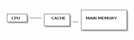
In a write through cache, every write to the cache causes a write
to main memory. This ensures that main-memory always contains the
latest version of any cached data, slows cache writes to the speed
of memory writes
In a write back cache, writes to cache locations are not immediately propagated to memory but are rather marked "dirty". When a "dirty" section is evicted form the cache it is written to memory. This allows faster cache writes, but can require two memory access to memory on a cache-miss (one to write out the dirty cache, and another to read in new content from memory). This also ensures less consistency guarantees.
-
log-structured file systems optimize writes. This is done by
buffering many small writes to the file system and writing them out
to one continuous section of disk. This turns small random-access
writes into fewer large contiguous writes allowing the write speed
of disks to approach the maximums supported by hardware.
in the log-structured file systems, data written at the same time is collocated, while in the Berkley FFS data belonging to the same file is collocated. So reading will be faster for the Berkley FFS as a whole file can read in fewer larger contiguous reads.
- skip TCP
-
consistency models – typically there is no global clock
- strong consistency
- (called sequential consistency in Munin paper) any write is immediately visible to subsequent reads
- causal ordering
- uses communication between processes to determine a global partial ordering – think Lamport clock
- weak consistency
- this is not really ever used. makes no guarantees that writes will be visible to future reads
- eventual consistency
- write will eventually be seen
- release consistency
-
uses two synchronization operators
release and acquire, either
- all writes are globally available after the writer releases the memory (i.e. eager)
- all writes are available to anyone who subsequently requires the memory (i.e. lazy also called entry consistency)
- PRAM consistency
- Pipelined Random Access Memory, also known as FIFO, writes are seen in the order they issue from the writer, which means that different processes could see different interleaved order of writes from different writers (only consistent order form a particular writer)
The main difference between weakened models like release consistency and entry consistency is that they allow for less coupling between processes. This reduces the communication overhead between processes. While strong and PRAM consistency provide more stringent guarantees simplifying the job of the developer they require much more work on the part of the OS.
-
In a write through cache, every write to the cache causes a write
to main memory. This ensures that main-memory always contains the
latest version of any cached data, slows cache writes to the speed
of memory writes
- section 3
-
using base-bound address space transformation instead of page
tables
this is simpler to implement, and takes less hardware (e.g. no TLB) and less transformations for memory lookup (no need to look into a page table for dereference). These are both appropriate for lower-power smaller embedded systems.
it looses some of the advantages of page tables, e.g. the ability to address large address spaces, the ability to load large programs into memory one-page at a time, and the ability to fight the fragmenting of main memory through regular page sizes. However with the smaller simpler programs running on these systems, and the lower degree of multiprogramming, these tradeoffs are generally in favor of base-and-bound addressing.
-
spin-locks "busy-wait" of sit on the CPU continually checking for
the lock to become available – this is ideal for locks which are
quickly aquire-able because it avoid the need for context
switching, however this is bad for low-wait locks as it wastes CPU
time.
blocking locks will yield the CPU to wait for a lock, placing the yielded process in a que for reactivation when the lock becomes free, this has the opposite benefits of spin locking.
with a highly bimodal distribution the introduction of a
max-spin-numbervariable could be used to spin for the time of the normal short lock, and then yield the CPU assuming the lock is of the longer variety. -
kernel designs
- monolithic
- fast in that all of the working components of the OS are already in kernel space, and they can share information and processes and communicate efficiently. this has the downside in that the kernel is large and complex, and it can be hard to develop new components.
- monolithic with loadable modules
- part way between monolithic and exokernel/library OS systems
- microkernels
-
the kernel is only responsible for process
separation and protection, in the case of L4
- address-spaces
- threads
- scheduling
- and synchronous inter-process communication
the micro kernel can do these simple things very quickly and efficiently, while still being easy to maintain. Also, having much of the functionality of the OS implemented outside of the kernel it makes the OS easier to maintain and extend.
having to push many system calls through the kernel-space user-space boundary multiple times (e.g. syscall for disk I/O, into kernel, then sent to disk driver in userspace, then back to kernel in kernel-space, then back out to OP)
- exokernels / library-systems
-
the kernel focuses on securely
multiplexing hardware resources between untrusted software,
and it makes these resources fully accessible to user-space
processes, so your device drivers are implemented entirely as
linked libraries in userspace, avoiding the need for many
user/kernel-space crossings
very easy to extend new functionality, in some ways faster than µ-kernels
not possible for separate drivers held in separate processes to cooperate.
-
using base-bound address space transformation instead of page
tables
- section 4
-
multiprocessor scheduling
- single global scheduler
-
easy to implement things like
barriers, easy to apply a global ordering on the scheduled
events in the system, easy to implement global scheduling
decisions and to avoid starvation, simple to program and to
reason about. All the information is in one place.
brittle, in that if this one proc breaks, then everything breaks until a new leader is elected
slow, this one proc could becomes a bottleneck
inefficient, this one proc may need to keep track of a very large number of jobs, leading to inefficient sorting of jobs by priority, etc…
needs large job quanta, parallelism needs to be at a high level (can't efficiently exploit low-level parallelism and/or cooperation)
can't scale past a certain number of processes simply because of length of proc. queue
- cooperating per-proc schedulers
-
would take load off of the
global scheduler addressing problems of the size of the
proc. queue on the global scheduler, and it's potential for
serving as a bottle neck (e.g. context switch requires network
I/O)
lose ability to enforce global ordering on tasks.
increased complexity
- scheduler hierarchy
-
more difficult to program/reason, must
divide task and resources into hierarchy
less privileged points (but still exist e.g. at the top of the hierarchy)
difficult to program and reason about
no single communication bottlenecks
smaller job quanta is possible
- how to implement a network FS with a simple processing switch at it's core
-
multiprocessor scheduling
- section 2
- Theory
- Exam Seating
Given a graph, can you order the nodes of the graph s.t. no two adjacent nodes in the ordering share an edge.Hamiltonian Path ⊆ Exam Seating
for any Hamiltonian Path take the compliment of the graph, and try to find an Exam Seating.
- flying between cities
not finished on the third part-
Djikstra's shortest path.
keep a sorted list of possible outgoing paths, at each iteration follow the lightest path in the list, and add the aggregate weights of the outgoing paths to the list.
This runs in time polynomial in the size of the graph – no edge will be traversed more than once.
- We can no longer track the shortest aggregate path (because length matters as well). So we can do this one through multiplication of the transition matrix. k multiplications runs in time polynomial in n but not in k.
- We can't do this in multiplications of the transition matrix. There are (n-1)k possible paths of length k. We can't sort these in polynomial time in either n or k.
-
Djikstra's shortest path.
- minimum weight spanning tree
minimum weight spanning tree.- check all cycles containing e.
- if e is the heaviest edge in any of those cycles, then it is not in the minimum weight spanning tree.
the first part can be done by incrementally stepping out along edges leaving e. as each edge is traversed check if it completes a cycle, and check if e is the max-weight edge in that cycle, this will take O(|E|) time.
- hash table
chance of log(n) items in one placekeep in mind that
- \(\binom{n}{k} \simeq \frac{n^k}{k!}\)
for any one bin \begin{eqnarray*} P(k) &=& \binom{n}{k}\left(\frac{1}{n}\right)^{k}\left(1-\frac{1}{n}\right)^{n-k}\\ &\leq&\frac{n^k}{k!}\left(\frac{1}{n}\right)^{k}\left(1-\frac{1}{n}\right)^{n-k}\\ &<& \frac{1}{k!} \end{eqnarray*} so for all bins
\(P(k) < \frac{n}{k!}\)with Sterling's approximation we can change this to
\(P(k) < \frac{n}{(\frac{k}{e})^{k}}\)so we'll want \(\left(\frac{k}{e}\right)^{k} > n\), which becomes true when we get k up to about ln(n)
- perfect matching
easy, every vertex which has different edge matchings is in the same cycle in each matching, and can transfer between the two graphs by rotating the cycling.if two graphs have many different edges in many different cycles, well then just do the cycles one-by-one.
- is NP-completeness relevant to the real world
not needed now- cryptography P=NP → cracking is as easy as decryption
- Exam Seating
Fall 2005
- OS
- short answer
-
deadlock is when no progress can be made in a system because more
than one process are all mutually holding resources needed by other
processes and are waiting for the freeing of resources needed by
other processes.
- mutual exclusion
- no preemption
- hold and wait
- circular wait
- the optimal page replacement strategy is to evict the page which will next be needed furthest in the future. This strategy is frequency approximated by LRU which assumes that the immediate future will resemble the immediate past
-
a journaling file system maintains a journal of all changes to
disk. In the event of a failure which would otherwise leave the
disk in an inconsistent state, rather than having to check all
inodes on disk the OS can step back to the last confirmed valid
point in the journal and replay all subsequent actions from there.
- how is this different from the journal OS
- ????
-
deadlock is when no progress can be made in a system because more
than one process are all mutually holding resources needed by other
processes and are waiting for the freeing of resources needed by
other processes.
- medium answer
- Caching
- Virtual Memory
- ???
- Policy and Mechanism in Modern OS
- design
- short answer
- PL
- Theory
Spring 2006
- Theory
- 7
transition matrix1/3 1/3 1/3 0 0 0 0 1/3 1/3 1/3 0 0 0 0 1/3 1/3 1/3 0 0 0 0 1/3 1/3 1/3 1/3 0 0 0 1/3 1/3 1/3 1/3 0 0 0 1/3 - eigenvector/eigenvalue pair
-
for a matrix A, the eigenvector x
s.t. A x = λ x where A is the eigenvector and λ is the eigenvalue
- A x = λ x
- [A x - λ x] = 0
- [A - λ I] x = 0 – where I is the identity matrix
- [A - λ I] x = 0 ⇒ det([A - λ I] x) = det([A - λ I])det(x) = 0
- determinant
-
sum of product along down-sloping diagonals minus sum product of up-sloping diagonals, so 1*4 + 2*3 - 1*4 - 2*3 = 01 2 3 4
so if det([A - λ I]) = 0, then we know [A - λ I] =
1/3 - λ 1/3 1/3 0 0 0 0 1/3 - λ 1/3 1/3 0 0 0 0 1/3 - λ 1/3 1/3 0 0 0 0 1/3 - λ 1/3 1/3 1/3 0 0 0 1/3 - λ 1/3 1/3 1/3 0 0 0 1/3 - λ and…
- (1/3 - λ)6 + (1/3)6 + (1/3)6 = 0
- (1/3 - λ)6 = 2(1/3)6
- (1/3 - λ) = (2(1/3)6)1/6
- 1/3 - λ = 21/6(1/3)
- λ = 1-21/6/3
- 7
Fall 2006
- PL
- 3.2 Axiomatic and Denotational Semantics – comparison
- denotational semantics
-
Formal basis is in set theory. State is
explicitly represented. A program is a mathematical functions
(the composition of many functions) from state to state.
Expressions return the value of some aspect of the state.
Statements are functions from state to state.
- axiomatic semantics
- More abstract than denotational semantics. Rather than explicitly representing state, we only track predicate statements about the state. A program transforms these predicates, and the semantics of a program are represented in terms of weakest preconditions and strongest postconditions of these predicates represented as Hoare triplets.
These semantics are similar in that they can both be used to track the effect of a program on state (with varying degrees of abstraction). Also both of these semantics break programs into side-effect-free expressions, and side-effect-full statements. The Axiomatic semantics of a program can be derived from the program's Denotational semantics.
There are cases in which each semantics could be preferable to another.
-
When working with an imperative program, in which some properties
(expressed in predicate logic) of the state are of interest
(e.g. invariants) and where program termination is of interest, then
Axiomatic semantics will be preferable.
For example the following program which returns the product of two positive inputs, will terminate and when it does a will be equal to the product of the inputs.
a = 0
b = INPUT1
c = INPUT2
while c > 0 do
  a = a + b
  c = c - 1
endwhile
a
Termination can be proved with the following space \(\mathbb{N}\), ordering $<$, and measure c, and the observation that c decreases under this measure with every loop iteration, shown with the weakest precondition across the while loop.
\begin{eqnarray*} \{Q\} c := c-1 \{P\}\\ Q &=& wp(c := c-1, P)\\ Q &=& P|^{c+1}_{c} \end{eqnarray*} so ∀ loop iterations the value of c decreases under the strict ordering described above.
Correctness can be shown with loop invariant $$b \times c + a = INPUT1 \times INPUT2$$
This can be seen trivially at the start of the loop because \(a=0\). This property is maintained through each loop iteration. \begin{eqnarray*} \{Q\} c := c-1 \{P\}\\ Q &=& wp(a=a+b; c:=c-1, P)\\ Q &=& P|^{c+1}_{c}|^{a-b}_{a}\\ \end{eqnarray*} our loop invariant remains true across this substitution \begin{eqnarray*} INPUT1 \times INPUT2 &=& b \times c + a|^{c+1}_{c}|^{a-b}_{a}\\ &=& b \times c + a - b|^{c+1}_{c}\\ &=& b \times (c+1) + a - b\\ &=& (b \times c) + b + a - b\\ &=& b \times c + a \end{eqnarray*} so when \(c=0\) then \(INPUT1 \times INPUT2 = a\).
- When working with a program which can be naturally decomposed into a series of function compositions then denotational semantics may be preferable, this is especially true if it is possible to reason mathematically about actions of the statements in the program on the state of the program.
- 3.2 Axiomatic and Denotational Semantics – comparison
Fall 2007
- OS
- section 2
- 1
- before 25
- before 34
- 2
7. Fall 2006 3.2 - 3
don't care - 4
sequential and causal consistency in a group RPC system- strict consistency
- everything happens in exactly the order in which it was sent – everything happens in the same order as if it was done by a single processor
- causal consistency
- events which potentially are causally related are seen by every node of the system in the same order
- 1
- section 3
- 1
- H
- F
- E
- D
- A
- B
- G
- C
- 2
12. Fall 2007 3.2 - 3
distributed hash table- servers organized in a logical ring
- every node maintains a table of the tables powers of two further along from itself down the ring of servers
- send a request to a server, it sends the request to the server in it's lookup table which is closest to and smaller than the destination
- 1
- section 4
- 1
- 2
- 1
- section 2
Spring 2008
- OS
- 4.2 VM
how to make a VM look convincingly like a real OS- fake everything and have virtual drivers living underneath all of the hardware drivers
How to detect if you are running inside of a VM
-
peg the CPU, and compare cpu-time to wall clock time, with knowledge
of the CPU and the OS it should be possible to calculate
- the instructions that should be executed on the CPU
- the wall-clock time it should take to execute the code
- the actual time it takes to execute the code
- time required for hardware access (e.g. memory) should be able to detect presence of the VM supervisor
- environmental factors, fan speed, cpu temperature monitors
- 4.3 Network Protocol Performance and Security
- send receipt packets even for packets you're not receiving
-
random IDs in the sent packets make it impossible to fake a receipt
- 4.2 VM
Fall 2008
- PL
- 3.3 Denotational and Axiomatic Semantics – application
A simple language with the following operations
is extended to include+ × - > ≥ if ∘ while Since expressions will now have side effects, we must change our denotational semantics. Both expressions and statements will now accept and return tupples of a value and a state <Val,St>, more formally they will be functions from tupples to tupples. In this way the state will explicitly pass through every expression and statement in a continuation passing style.
So, for example the denotational semantics of the id operator will become (using the convention where Val refers to the first element of the argument tupple, and St refers to the second element of the argument tupple). $$\llbracket id \rrbracket =
All of the primitive operators can be encoded in the following manner.
Note that the commutativity of our arithmetic operators is now broken, since either expression could change the state and thus change the value of the subsequent expression.
The new operators can be encoded as.
Finally the if and while operators can be encoded as.
The Axiomatic Semantics can be derived from the Denotational Semantics. Assignment \(x := e\) must now take into account the effect of the expression on the state. \begin{eqnarray*} \{Q\} x := e \{P\}\\ wp(x := e, P) &=& wp(e, P)|_{x}^{e_{val}} \end{eqnarray*}
- 3.5 fixpoint semantics
- Pa
- add(0,x,x) :- nat(x).
- add(s(x),y,s(z)) :- add(x,y,z).
- inc(x,y) :- add(x,s(0),y).
- nat(0).
- nat(s(x)) :- nat(x).
Calculation of fixed point
- TP0(∅) = nat(0) (0.0) from 4
-
TP1(∅) = TP(TP0)
- nat(s(0)) from 5 applied to 0.0 (1.0)
- add(0,0,0) from 1 applied to 0.0 (1.1)
-
TP2(∅) = TP(T1)## with x=s(0)
- nat(s(x)) from 5 applied to 1.0 (2.0)
- add(0,x,x) from 1 applied to 1.0 (2.1)
- add(x,0,x) from 2 applied to 1.1 (2.2)
-
TP3(∅) = TP(TP2) ## with x = s(0)
- add(s(0), x, s(x)) from 2 applied to 2.1 (3.0)
- inc(0,x) from 3 applied to 2.1 (3.1)
-
TP4(∅) = TP(TP3) ## with y=s(x)
- inc(x,y) from 3 applied to 3.2 (4.0)
- fixed point
- Pb
- add(0,0,0).
- add(s(A),0,s(A)) :- nat(A).
- add(A,s(B),s(C)) :- add(A,B,C).
- inc(0,s(0)).
- inc(s(A),s(B)) :- inc(A,B).
- nat(0)
- nat(s(x)) :- nat(x)
Calculation of fixed point
-
TP0(∅) =
- add(0,0,0) from 1 (0.0)
- inc(0,s(0)) from 4 (0.1)
- nat(0) from 6 (0.2)
-
TP1(∅) = TP(TP0)
- …
- Pa
- 3.3 Denotational and Axiomatic Semantics – application
Spring 2009
- Theory
theory09.pdf - OS
- short answer
- in the Chord what is the purpose of the finger table – to index the next ln(n) neighbors
- pid in a TLB is useful so you don't have to flush the TLB entirely when you context switch, instead you can flush entry by entry
-
RISC can run at a higher clock speed because the instructions are
closer to the hardware, CISC can do more with one instruction but
the clock could be slower
runtime = Instructions × Cycles/Instruction × Sec/Cycle
also, due to increased complexity, CISC instructions could be harder to parallelize on the instruction level
-
bridges connect networks, and learning bridges remember the
shortest path to individual machines
bridges connect networks, at first they just flood broadcasts, but once they learn where something is they target their output
- medium answer
-
If I/O bound processes have a higher priority they will be on and
off of the CPU quickly, increasing the total resource usage by
keeping the I/O devices busy.
On a user system this will also increase "responsiveness" of the machine, but pushing through processes which interact with the users (screen or keyboard are both I/O devices).
- Multimedia tends to have a lot of large streaming writes and reads which means that a contiguous series of blocks will be written at once. With these large streaming I/Os there is less need for parallel access, and you'd rather have your parity bits out of the way of your reads/writes.
- shared memory through message passing. each page lives on a single machine, and it's writes are broadcast to other machines reading that page.
-
If I/O bound processes have a higher priority they will be on and
off of the CPU quickly, increasing the total resource usage by
keeping the I/O devices busy.
- long answer
-
TCP traffic between cities
- traffic engineering
- conscious adjustment of traffic to avoid busy times of day
- route flutter
- slight variations in packet headers can change the intermediate routers used
- diurnal patterns
- measure at different times of day, (email in morning, and then at night when you get home etc…)
- asymmetries
- route there could be different from route back, also maybe producers and consumers of information are not evenly distributed between countries
-
with >32 node systems what are the advantages of running separate
kernels on separate processors
- disadvantages
-
increased communication overhead for
implementing distributed consistency
a lock could be more difficult, disabling interrupts doesn't help when other kernels still have active threads which could try to use your resource
sharing resources between kernels (e.g. one large external disk) would be difficult (you would need a kernel of kernels)
(see Quicksilver)
if you have to pass a big message, you just write the message out to a place in memory and pass around the address. Kernels could similarly respond to a message by writing to a place in shared memory
leader election is the process of designating a single process as the organizer of some task between separate computers
again we could our "each kernel has a designated place in memory" trick to allow nodes to communicate between memory writes.
-
TCP traffic between cities
- short answer
- PL
build up with TP
Questions by Topic
file system
- Jan 2009 3.2
- Jan 2008 3.2
- Aug 2006 2.1 4.2
- Jan 2006 2.3
- Aug 2005 2.3
- Jan 2005 2.2
- Spring 2004 3.3
- Aug 2003 3.3
- Aug 2001 1.2,1.3 1.4
- Jan 2001 1.1
NP-Completeness
- Spring 2009
- 3
NP-completecan reduce Hamiltonian path to k-leaf spanning tree
2-leaf spanning tree ≡ Hamiltonian path
- TODO 6
dynamic programmingnot all graphs are trees so this doesn't mean that P=NP
- 7
This is ∈ P because there are only two choices for each vertex, so it's like 2-SAT.
- 3
- Fall 2007
- 1 (widget salesman)
- like traveling salesman, but not
- vertices weighted with different values for different days
think of this as a large directed graph with weighted vertices, each city/day combo gets a vertex, directed edges allow traversal through the graph moving forward in time.
dynamic programming
like the beach-front property problem in the HW
time and space
- this would take polynomial time thanks to dynamic programming
- this would take exponential space – because you would need to store the answer for each subset of the graph
(defn travel [s G W]
  (max (map
        ;; where t is the node landed on by that edge
        (fn [t] (+ (:value t) (travel t G W)))
        (edges-leaving-to s G))))
- 4
DNF is in Pconverting from CNF to DNF, you get an exponential number of clauses
- DONE 5
I think this would be a regular language. This is true because the state is always finite.We say that u ∼ v if ∀ w : uw ∈ L ⇔ vw ∈ L, if a language has a finite number of equivalence classes under ∼, then it is regular
Lets say that u ∼ v iff the set of the last two digits of the possible predecessor strings of u and v are equal. It is clear that if this is the case, then u and v satisfy the ∼ property. The number of such sets is finite, because 22=8 possible strings of two bits and 64 possible states. \(\square\)
how about for a two dimensional tiling?
- intuition says it should work
- apparently wikipedia says otherwise
- 1 (widget salesman)
- Spring 2007
- 1 (shore-front property)
- TODO 2
take 1/edge-weight for each edge weight and then run minimum spanning tree - DONE 3
dynamic programming, working from right to left along the sequencethese would take nlgn space, n subsequences which need to be tracked, and each subsequence has a number of size n (taking up lg(n) space)
6 2 17 4 9 8 10 5 12 (defn rests [lst] (if (empty? lst) '() (cons lst (rests (rest lst))))) (defn mymax [lst] (if (empty? lst) 0 (apply max lst))) (memoize (defn inc-subseq [lst] (if (empty? lst) 0 (let [me (first lst)] (inc (mymax (map inc-subseq (filter #(< (first %) me) (rests (rest lst)))))))))) (inc-subseq nums)
and in emacs-lisp
(defvar my-cache '())

(defun inc-subseq (lst)
  (or (cadr (assoc lst my-cache))
      (if (= (length lst) 0)
          0
        ((lambda (answer) (setq my-cache (cons (list lst answer) my-cache)) answer)
         (+ 1 (apply #'max
                     (cons 0 (maplist
                              (lambda (el)
                                (inc-subseq (when (< (car el) (car lst)) el)))
                              (cdr lst)))))))))

(inc-subseq (reverse '(6 2 17 4 9 8 10 5 12)))
- 4
- optimal solution
- place three connected nodes off to the side
- connect two of the three to one node – thereby forcing it to have a color
- ∀ remaining nodes in the graph, continually connect it to two of the three in our floating triangle until one of the solutions is colorable – thereby forcing a coloring for that node
this will take at most 3n time

- suboptimal solution
- pick a node at random and call it red (without loss of generality)
- ∀ other nodes, connect those nodes to the selected node, and ask if the remaining graph is still 3-colorable, if not, then the newly selected node is also red
- after n questions we know all of the red nodes
- we then do the same thing for green and blue
after at most 3n questions we have found all of the red, green, and blue nodes
there could be some nodes left over
- optimal solution
- DONE 6
first we can check a witness can be checked in polynomial time, ∀ corner we check that the rectangle at that corner doesn't overlap the nearest corners – like O(n2) or solook at p.153 in the book, also maybe p.178
maybe this is equal to integer partition or subset sum
if integer partition is NP-complete, then cool can do the following
let every little rectangle have unit height, and the big rectangle have height of 2 units, tiling is the same as the partition problem
if we're scared of rotation, then we can just size our rectangles such that the smallest length is greater than 2
- 1 (shore-front property)
- Fall 2006:
- 1
Just take nodes out one at a time and then ask "does there still ∃ an independent set of size k".notes
- independent set converts to vertex cover
- independent set converts to clique in the complement of the graph
- 3
A counter which increments for each "(" and decrements for each ")", then the counter would be in Ω(log(n)).An example of a string which can't fit into o(log(n)) would be the string of n "("s, because with the last "(", the counter would hit it's max and cycle back to 0.
- 4
- turn every vertex into a triangle, converts from 3-coloring → equal 3-coloring
for these types of problems we need to
- show that the conversion can be done in polynomial time
- show that we can map yes instances to yes instance and no instance to no instance
- 6
If P=NP then we can collapse quantifiers ∃ and ∀, the entire polynomial hierarchy collapses and we the encrypt crypto and the decrypt crypto problem become equal (and easy)
- 1
- Spring 2005, 1, 2, 3, 6.
typing
- Jan 2009
- 3.1
did (1) and (2) w/pencil and paper.for (3) it's not as clear how to handle variant types, also, what is meant by "sums"
- TODO 3.2
need to talk to Darko
- 3.1
- Aug 2008 3.1, 3.2 (Same as 2009)
- Jan 2008
- TODO 1.3 (Simple type lambda calculus)
look up erasure – once I have the book… - spring 08 1.4
-
division by 0
f 3
    where
      f x = x `div` 0
lets say that
divhas type Int → Int → Maybe Int, then f x has type Int → Maybe Int, and more specifically becausefalways divides by 0 it has type Int → Nothing, so the type of the entire expression is Nothing -
f 3 where f x = xhas type Int, because f has type a → a, and x is an Int -
(f x, f "a")again f has type a → a, sof 3has type Int andf "a"= has type String, and there tuple then has type =(Int, String) -
in the following
f g [[1],[2,3]]
    where
      f h = map (map h)
      g n = n * n
we can assign the following types
map :: (a -> b) -> [a] -> [b]
f :: (a -> b) -> [[a]] -> [[b]]
g :: Num a => a -> a
so the composition of f and g has type
Num a => [[a]] -> [[a]] which when applied to an item of type =[[Int]]= results in a an item of
the same type
-
the following "i believe" should fail with a recursive type issue
f g [[1],[2,3]]
    where
      g :: Num a => a -> a
      g n = n * n
      twice :: (a -> a) -> a -> a
      twice f a = f (f a)
      f :: (a -> a) -> -- fails to have a type, infinite recursive type
      f h = twice map h
discuss what choices the language designers made, and what would results from stricter and/or from less strict polymorphism.
-
division by 0
- 3.3
lookup let polymorphism, and polymorphic functionsusing let it can be possible for a polymorphic function to be used with multiple different, so for example id (λ x . x) is fully polymorphic, and the following could work where id is applied to objects of two different types (a function and a natural number)
let id=(λ x . x) in
(id (λ k . "this")) (id 5)
the above works because the type of id is calculated to be polymorphic during evaluation of the head of the let before the body of the let, however the following will not work, because the type of id is first calculated to be a function on functions (λ k . k), and then it can't be re-applied to 5 (a number)
(λ id . ((id(λ k . k))(id 5)))(λ n . n)
This could be resolved through declaration of polymorphic functions
- TODO 1.3 (Simple type lambda calculus)
- Aug 2007 1.6 (ML)
(see spring 08 1.4) - Jan 2007 1.1 (SML)
- Aug 2006
- 1.3 (ML)
(see spring 08 1.4) - TODO 3.1 (lambda calculus)
- (if x (succ 0) (iszero y))
-
if e is typable with type Τ and f is a normal form of e, then
f has the type of Τ.
the evaluation rules of λ-calculus preserve type, an expression which does not have a normal form does not have a type
- 1.3 (ML)
- Jan 2005
- 1.4 (ML type-correctness)
- 1.5 (ML Type reconstruction)
- 3.3 (type-correct)
- 1.4 (ML type-correctness)
- Spr 2004 3.3
- Jan 2003
- 1 (ML Type reconstruction)
- 7 (static semantic of an explicitly-typed core)
- 1 (ML Type reconstruction)
- Aug 2003 1.2.2 (SML) 1.3.1 (SML)
axiomatic and denotational semantics
(for axiomatic semantics see cs550-notes)
wikipedia is actually a pretty good resource for this
- Spring 2009: 3.3, 3.4
- 3.3
in a simple programming language with +, *, -, <, ≥, assignment, conditionals, sequencing and while loops, and side effect free expressionswe add ++ and – (both prefix and postfix) to the language, what changes in the semantic rules of the language (consider both axiomatic and denotational).
With the addition of these rules the language no longer has side effect free expressions. Now essentially all language constructs which rely on the side-effect free nature of expressions (i.e. a conditional assuming that it's guard doesn't change state) will need to be updated to explicitly allow expressions to affect state.
give an example of a guarded if statement with both a side-effect free expression in the guard, and with a potentially active expression in the guard.
-
denotational semantics
- [if b then s1 else s2] = [b] → [s1] else [s2]
- becomes
- [if b then s1 else s2] = ([b] → [s1] else [s2]) o [b]
- we can then break all other language constructs down into instances of the if and loop, where loop isn't affected by this change
-
axiomatic semantics
-
wp(if b then s1 else s2, α) = β, so
- β ∧ b → wp(s1,α)
- β ∧ ¬ b → wp(s2,α)
- becomes
-
wp(if b then s1 else s2, α) = β, so
- β ∧ b → wp(s1,wp(b,α))
- β ∧ ¬ b → wp(s2wp(b,α))
-
wp(if b then s1 else s2, α) = β, so
-
denotational semantics
- 3.4
- structural operational semantics
- Analysis of the meaning of a program as the series of operations which constitute the programs evaluation. These operations can be constructed as if → then rules of evaluation. (see operational semantics)
- natural semantics
- ?
- denotational semantics
-
explicit state, and the meaning of a
program is a mathematical function, foundational basis is
set-theory, program is a mathematical function from state to
state.
- expressions
- don't have side effects
- statements
- have side effects
- axiomatic semantics
- programs operate on formulas specifying properties of state, the semantics of a program is the effect of the program on the strongest properties of the states
- 3.3
- Fall 2008: 3.3 (same as S09 3.3), 3.4 (very similar to S09 3.4)
- Spring 2008: 3.1, 3.2 (same as F08 3.4)
- Fall 2007: 3.1, 3.2 (indirectly)
- Spring 2007: 3.3, 3.4.1 (same as S09 3.4)
- Fall 2006: 3.2 (same as S09 3.4)
- Spring 2006: 3.2 (same as S09 3.4)
- Fall 2005: 3.2
- Spring 2005: 3.1 (same as S07 3.3), 3.2 (same as S09 3.3)
probability
- TODO Spring 2009: 5
how many n items can we fit into an m place hash before we start to see collisionswe know that when \(n = \Theta(\sqrt{m})\) we start to see collision
how big can n be in relation to m before we start to see collisions
\begin{math} \binom{n}{3} \times \frac{1}{m^3} \geq 1 \end{math} \(\binom{n}{k}\) is always roughly equal to \(\frac{n^k}{k!}\)answer is \(m^{\frac{2}{3}}\)
- Fall 2007: 3, 7.
\(\frac{1}{3}\left(\left(\frac{-1}{2}\right)^n \frac{2}{3} \right)\) - Spring 2007: 7
-
p(k-1|k) will be
give a kumquat (k)/3 receive not a kumquat (k)/3 -
p(k+1|k) will be
give not a kumquat receive a kumquat -
p(k|k)
give and get kumquat give and get not-kumquat
-
p(k-1|k) will be
- Spring 2005: 4
n elements in an n-space hash, with high probability no space has log(n) elements- see 07-hashing.pdf
keep in mind that
- \(\binom{n}{k} \simeq \frac{n^k}{k!}\)
fixed points
- Spring 2009: 3.5
looks like whilerev1andrev2are true for the same input sets, the two programs are not fully equivalent through fixed point analysis.- lets pick the naturals for our atoms
-
we start applying TP to this domain for a couple of steps,
- first just everything which doesn't have a body
- then build up on those, body → head, etc…
-
eventually maybe prove inductively that ∀ sets which satisfy
rev1, those same sets will also satisfyrev2, start with empty trivial sets and grow from there
- Fall 2008 : 3.5
This says compute the fixed point semantics, while 3.6 says compute the logical semantics, what's the difference given that the meaning of a logic program is that program's minimal fixed point. Aren't these equal?fixed point semantics is
- start with empty (just the ground terms)
- begin applying TP building up successive sets
- Spring 2008: 3.4
- Fall 2007: 3.3
- Jan 2007: 3.1
- Fall 2006 : 3.3
- Jan 2006 : 3.3
- fall 2005 : 3.3
prolog questions
- Jan 2009: 1.5
- the second is a "continuation passing" version of the first, in which the state of the computation is explicitly passed between functions.
-
possible stack trace?
natlist([0, s(0)], write('success!'))
nat(0, natlist([s(0)], C))
nat(0, nat(s(0)), natlist([], write('success!')))
nat(0, nat(s(0)), call(write('success!')))
nat(0, nat(s(0)), TRUE)
nat(0, TRUE)
TRUE
output of
natlist([], C) :- call(C).
natlist([X|T], C) :- nat(X, natlist(T, C)).

nat(0, C) :- call(C).
nat(s(X), C) :- nat(X, C).
on
natlist([0,s(0)],write('success')).yields
?- natlist([0,s(0)],write('success')).
success
true.
and
natlist([]).
natlist([X|T]) :- nat(X), natlist(T).

nat(0).
nat(s(X)) :- nat(X).
on
natlist([0,s(0)]), write('success').yields
?- natlist([0,s(0)]), write('success'). success true. -
implement a parser to do this
%% matches prolog clauses, and write out their continuation versions
cont([]).
cont(A,B) :- write(A), bodycont(B).

%% matches the body of a clause, and writes out a continuation version
bodycont(B) :- %% only one clause, then print it w/continuation arg.
        not 'C'(B,b_first,',',b_rest,')'),
        not 'C'(B,b_inside,')'),
        write(B), write(b_inside) write(',C)').
bodycont(B) :- %% multiple arguments, then recurse
        'C'(B,b_first,',',b_rest),
        write(b_first), write(','), bodycont(b_rest).
- Aug 2008: 1.3
same as above (binarized) - Jan 2008: 1.1
-
write a program to translate roman numerals
%% lookup values of the numbers
value('I',1).
value('V',5).
value('X',10).
value('L',50).
value('C',100).
value('D',500).
value('M',1000).
value(A,B,N) :- value(A,M), value(B,O), >=(M,O), plus(M,O,N).
value(A,B,N) :- value(A,M), value(B,O),  <(M,O), plus(N,M,O).

%% values for strings of characters
roman([],0).
roman([A],U) :- value(A,V), =(U,V).
roman([X,Y|Rest],U) :-
        value(X,Xval), value(Y,Yval), >=(Xval,Yval),
        roman([Y|Rest],V), plus(Xval,V,U).
roman([X,Y|Rest],U) :-
        value(X,Xval), value(Y,Yval), <(Xval,Yval),
        roman([Y|Rest],V), plus(U,Xval,V).
some notes on the above
-
there is no
minusin prolog, you only needplus - keep in mind the difference between "," and "|" when dealing with lists.
- two functions are needed to differentiate between the literal lookup value of a letter, and it's actual contribution to the total of the whole numeral.
-
there is no
-
can this program be "run backwards" to subtract roman numerals?
If it means subtract as in "-" the arithmetic operation on numbers, well then no, this translates from numerals (i.e. strings of characters), to the actual abstract platonic ideals which are numbers (i.e. quantities). This program could not be used to manipulate quantities, only to translate from character strings to quantities.
However the program can be used to generate numerals from quantities, however these would not necessarily be constructed as the Romans would have done, e.g.
roman(Numeral,1972).
Numeral = ['I','I','I','I'...]
however with some length restriction there are interesting results.
?- roman(['I', 'I', 'I', 'I', 'L', 'M', 'M', 'X', 'X'] , M).
M = 1972
-
write a program to translate roman numerals
- Jan 2008 1.2
same as above (binarized)
λ-calculus questions
- 1) Spring 2009 2.1
α-normalization is the primary means of evaluation in the λ-calculus. It is the process of recursively applying β-reductions to a λ-expression until it either reaches a normal form, or diverges or falls into an infinite loop indicating that ¬∃ a normal form.a meaningful example – summation of church numerals 1 + 2
;; +
λ m n. λ f x. (n f m f x)
;; 1
λ f x. (f x)
;; 2
λ f x. (f (f x))
β-reduction
λ n. λ f x. (n f (λ f x. (f x)) f x)
;; 2
λ f x. (f (f x))
β-reduction
λ n. λ f x. (n f (f x))
;; 2
λ f x. (f (f x))
β-reduction
λ f x. (λ f x. (f (f x)) f (f x))
β-reduction
;; 3
λ f x. (f (f (f x)))
- 2) Fall 2008 2.2 (Same Question as 1)
- 3) Fall 2008 1.3
- 4) Spring 2008 2.2 (Same as 1 and 2)
- 5) Spring 2008 3.3
write down the evaluation and typing rules for the pure call-by-value λ-calculusfirst lets fully define our simply-typed call-by-value λ-calculus with the following abstract syntax
t ::=
    c, an atom
    v, a variable
    (t,t), an application of two terms
    (\lambda x. y), a \lambda expression where x is a variable and y is a term
    let x=t in y, x is var, t and y are terms
    x \rightarrow y; z, where x y and z are terms
    primop, t_1, t_2, etc... where t_i are all terms and primop is a primitive
evaluation
- application
- (a b) if a is a λ expression (e.g. (λ x. e)) then pass b to a or [x → b]e
- if
-
the following is
strictin t and islazyin t1 and t2, meaning if t is \(\bot\) then the whole statement is also, but not necessarily so for t1 and t2- if true then t1 else t2 → t1
- if false then t1 else t2 → t2
- \(\frac{t \rightarrow t'}{if t then t_1 else t_2 \rightarrow if t' then t_1 else t_2}\)
- ???
- β-reduction
typing
- true : bool
- false : bool
- 0 : nat
- \(\frac{t_1 : nat}{ succ(t_1) : nat}\)
- \(\frac{t_1 : nat}{ pred(t_1) : nat}\)
- \(\frac{t_1 : bool, t_2 : T, t_3 : T}{if t_1 then t_2 else t_3}\)
- 6) Spring 2006 3.1
-
normal forms
-
- ((λ (x) (λ (y) (x (λ (x) x)))) (λ (y) (x y)))
- (λ (y) ((λ (y) (x y)) (λ (x) x)))
-
(λ (y) ((x (λ (x) x))))
- ((λ (x) (y (λ (v) (x v)))) (λ (y) (v y)))
- (y (λ (v) ((λ (y) (v1 y)) v)))
- (y (λ (v) ((v1 v))))
-
-
type checking
;; g :: [a -> b] -> [[a] -> [b]]
(define g (lambda (f)
            (lambda (l)
              (if (null l)
                  nil
                  (cons (f (f (car l)))
                        ((g f) (cdr l)))))))
;;        cdr     :: [a] -> [a]
;;     (g cdr)    :: [[a]] -> [[a]]
;;  (g (g cdr))   :: [[[a]]] -> [[[a]]]
;; ((g (g cdr) l) :: [[[a]]]
((g (g cdr)) l)
-
lis a list of any type -
gand(g (g cdr))are functions with the types shown above whereacan be any type
-
-
fixed points
(define F (lambda (f)
            (if (= x 0)
                1
                (if (= x 1)
                    2
                    (+ (f x)
                       (f x)
                       (neg (f (- x 1))))))))
the least fixed point would be the function f defined by the following table.
this is the only, and also the least fixed point of this function.input output \(\bot\) \(\bot\) 0 1 1 2 \(\bot\) \(\bot\) \(\vdots\) \(\vdots\) - ¬∃ any lesser fixed points
- assume ∃ g s.t. g is less than f and g is a fixed point of F. Then either g(0) < f(0), or g(1) < f(1) because everywhere else f is \(\bot\), this is a contradiction, because if either of the above cases is true, then F(g) ≠ g and g is not a fixed point, similarly
- ¬∃ any /greater fixed point
- assume ∃ g s.t. g is greater than f and g is a fixed point of F. Since g is a fixed point we know it's values for inputs of \(\bot\), 0 and 1, so ∃ n>1 s.t. g(n)≠\(\bot\), however this is a contradiction, because ∀ n>1 and ∀ functions h F(h)(n) = \(\bot\), because it calls F(h)(n).
so f is both the minimal and unique fixed point of F
-
normal forms
- 7) Fall 2006 3.1
-
give an example of a λ-expression without a type
if t1 then 0 else FALSE
this can't be typed because it's type could vary based on the value of t1, however this could still be part of a λ-expression which evaluates cleanly
- if e has type Τ and f is a normal form of e, then f is also well typed and has a normal form of Τ. This is true because all evaluation rules in the λ calculus preserve the type of well-typed expressions – I guess I could write them out, for this just pl-spring08-3.3.
- while every expression e has a unique normal form, it is possible that some paths of evaluation of e terminate while others do not → it is possible that ∃ e s.t. e is not typable because some paths of evaluation of e don't terminate, but those paths of evaluation from e that do terminate into a normal form (f) which could be typeable
- (see above pl-spring06-3.1)
-
give an example of a λ-expression without a type
- 8) Fall 2006 3.2 (Combined with 7)
this isn't λ-calculus, but it looks tough (see fall-06-3.2) - 9) Spring 2005 3.1
- 10) Fall 2005 1.6
- 11) Fall 2005 3.3
- 12) Spring 2004 3.3
haskell questions
- permute
permute :: Eq a => [a] -> [[a]]
permute [] = [[]]
permute a = foldr (\ x rest -> (map (\ tail -> x:tail) (permute (less x a)))++rest) [] a
    where
      less x ys = [y | y<-ys, not (y == x)]
in a different way
rem_dups :: (Eq a) => [a] -> [a]
rem_dups = foldr (\ x a -> if elem x a then a else x:a) []

permute :: (Eq a) => [a] -> [[a]]
permute [] = [[]]
permute a = concat $ map (\ x -> map (x:) $ permute $ less x a) $ rem_dups a
    where
      less x ys = [y | y<-ys, not (y == x)]
- just looking at primes – not from a test
sieve of Eratosthenes – taken from en.literateprograms.orgmodule Main( main ) where import System( getArgs ) primes :: [Integer] primes = sieve [2..] where sieve (p:xs) = p : sieve [x|x <- xs, x `mod` p > 0] main = do args <- getArgs print $ show(take (read (head args)) primes)
results in a script which take a number and prints out the first that many primes
now a faster version
module Main( main ) where
import System( getArgs )

merge :: (Ord a) => [a] -> [a] -> [a]
merge xs@(x:xt) ys@(y:yt) =
  case compare x y of
    LT -> x : (merge xt ys)
    EQ -> x : (merge xt yt)
    GT -> y : (merge xs yt)

diff :: (Ord a) => [a] -> [a] -> [a]
diff xs@(x:xt) ys@(y:yt) =
  case compare x y of
    LT -> x : (diff xt ys)
    EQ -> diff xt yt
    GT -> diff xs yt

primes, nonprimes :: [Integer]
primes    = [2, 3, 5] ++ (diff [7, 9 ..] nonprimes)
nonprimes = foldr1 f . map g . tail $ primes
  where
    f (x:xt) ys = x : (merge xt ys)
    g p         = [ n * p | n <- [p, p + 2 ..]]

main = do
  args <- getArgs
  print $ show(last (take (read (head args)) primes))
- spring 09 1.1
hungry hungry haskelldata Hungry a = T | H (a -> Hungry) hhh :: Int -> Hungry hhh 0 = id hhh n = const (hhh (n-1))
crazy data type
data A a = a -> A
- spring 09 1.2
matrix multiplication – can be done in language of choiceC11 = M1 + M4 − M5 + M7 C12 = M3 + M5 C21 = M2 + M4 C22 = M1 − M2 + M3 + M6
s.t.
M1 = (A11 + A22 ) · (B11 + B22 )
M2 = (A21 + A22 ) · B11
M3 = A11 · (B12 − B22 )
M4 = A22 · (B21 − B11 )
M5 = (A11 + A12 ) · B22
M6 = (A21 − A11 ) · (B11 + B12 )
M7 = (A12 − A22 ) · (B21 + B22 )
working in clojure
(defn mm [a b]
  (if (= (count a) 1)
    (list (list (* (first (first a))
                   (first (first b)))))
    (let [size (/ (count a) 2)
          fslice (fn [m] (map #(take size %) m))
          bslice (fn [m] (map #(drop size %) m))
          m+  (fn [a b] (map #(map + %1 %2) a b))
          m-  (fn [a b] (map #(map - %1 %2) a b))
          a11 (fslice (take size a))
          a12 (bslice (take size a))
          a21 (fslice (drop size a))
          a22 (bslice (drop size a))
          b11 (fslice (take size b))
          b12 (bslice (take size b))
          b21 (fslice (drop size b))
          b22 (bslice (drop size b))
          m1  (mm (m+ a11 a22) (m+ b11 b22))
          m2  (mm (m+ a21 a22) b11)
          m3  (mm a11 (m- b12 b22))
          m4  (mm a22 (m- b21 b11))
          m5  (mm (m+ a11 a12) b22)
          m6  (mm (m- a21 a11) (m+ b11 b12))
          m7  (mm (m- a12 a22) (m+ b21 b22))]
      (concat (map concat
                   ;; c11
                   (m+ (m- (m+ m1 m4) m5) m7)
                   ;; c12
                   (m+ m3 m5))
              (map concat
                   ;; c21
                   (m+ m2 m4)
                   ;; c22
                   (m+ (m+ (m- m1 m2) m3) m4))))))

(def a
     '((1  2  3  4)
       (5  6  7  8)
       (9  10 11 12)
       (13 14 15 16)))

(def b
     '((1  2  3  4)
       (5  6  7  8)
       (9  10 11 12)
       (13 14 15 16)))

(mm a b)
working in Haskell
mdo :: (Num a) => (a -> a -> b) -> [[a]] -> [[a]] -> [[b]]
mdo f a b = map (\ (x,y) -> (map (\(l,r)->l`f`r) (zip x y))) (zip a b)

mm :: (Num a) => [[a]] -> [[a]] -> [[a]]
mm [[a]] [[b]] = [[a*b]]
mm a b = (map (\ (x,y) -> x++y) (zip c11 c12))++
         (map (\ (x,y) -> x++y) (zip c21 c22))
    where
      c11 = mdo (+) (mdo (-) (mdo (+) m1 m4)  m5) m7
      c12 = mdo (+) m3 m5
      c21 = mdo (+) m2 m4
      c22 = mdo (+) (mdo (+) (mdo (- ) m1 m2) m3) m6
      m1 = mm (mdo (+) a11 a22) (mdo (+) b11 b22)
      m2 = mm (mdo (+) a21 a22) b11
      m3 = mm a11 (mdo (-) b12 b22)
      m4 = mm a22 (mdo (-) b21 b11)
      m5 = mm (mdo (+) a11 a12) b22
      m6 = mm (mdo (-) a21 a11) (mdo (+) b11 b12)
      m7 = mm (mdo (-) a12 a22) (mdo (+) b21 b22)
      a11 = map (take size) (take size a)
      a12 = map (drop size) (take size a)
      a21 = map (take size) (drop size a)
      a22 = map (drop size) (drop size a)
      b11 = map (take size) (take size b)
      b12 = map (drop size) (take size b)
      b21 = map (take size) (drop size b)
      b22 = map (drop size) (drop size b)
      size = (round ((fromIntegral (length a))/2))

-- [[1, 2, 3, 4], [5, 6, 7, 8], [9, 10, 11, 12], [13, 14, 15, 16]]
- DONE spring 09 1.3 (Haskell BFS)
(see annotated Haskell BFS)data Tree a = E | T a (Tree a) (Tree a) deriving Show -- so much easier than bfs dfnum :: Tree a -> Tree Int dfnum a = fst(dfn(a,1)) where dfn :: ((Tree a), Int) -> (Tree Int, Int) dfn (E,n) = (E,n) dfn (T _ left right, n) = (T (snd l) (fst l) (fst r), (snd r)) where l = dfn(left, n) r = dfn(right, ((snd l) + 1))
data Tree a = E
            | T a (Tree a) (Tree a)
              deriving Show

bfnum :: Tree a -> Tree Int
bfnum t = (head (bfn([t],1)))
    where
      bfn :: ([Tree a], Int) -> [Tree Int]
      bfn ([],_) = []
      bfn (trees,n) =
          bfcomb n trees (bfn (next_trees, ((round((fromIntegral(length next_trees))/2))+n)))
              where
                next_trees = (foldr (\ t a -> case t of E->[]++a; T _ l r->[l,r]++a;) [] trees)
      bfcomb :: Int -> [Tree a] -> [Tree Int] -> [Tree Int]
      bfcomb n (E:ts) rs               = [E] ++ (bfcomb n ts rs)
      bfcomb n (T _ _ _:ts) (r1:r2:rs) = [T n r1 r2] ++ (bfcomb (n+1) ts rs)
George's BFS
bfnum :: Tree a -> Tree Int
bfnum t = head $ q 1 [t]
q :: Int -> [Tree a] -> [Tree Int]
q _ [] = []
q i ts = dq (num i ts) (q n $ concat [[l, r] | T a l r <- ts])
  where dq [] _ = []
        dq (T i _ _:hs) (l:r:lrs) = T i l r:-Dq hs lrs
        dq (E:hs) (lrs) = E:-Dq hs lrs
        num k (T _ _ _:tl) = T k E E:num (k+1) tl
        num k (E:tl) = E:num k tl
        n = length [a | T a _ _ <- ts] + i
George's even shorter BFS
data Tree a = E
            | T a (Tree a) (Tree a)
              deriving Show

bfnum :: Tree a -> Tree Int
bfnum t = head $ q 1 [t]
    where q i ts = dq i ts (q (i + length [a | T a _ _ <- ts])
                             (concat [[l, r] | T a l r <- ts]))
          dq i (T _ _ _:hs) (l:r:lrs) = T i l r:dq (i+1) hs lrs
          dq i (E:hs) (lrs) = E:dq i hs lrs
- TODO spring 09 1.4
prove that scanl as defined herescanl :: (b -> a -> b) -> b -> [a] -> [b] scanl f e = map (foldl f e) . inits inits :: [a] -> [[a]] inits [] = [[]] inits (x:xs) = [] : map (x:) (inits xs)
runs in O(n2) time. Then give the definition of another function (scanl') which is more efficient.
There are many redundant computations. We foldl over the subsequences in inits which, however these elements are nested subsequences, so for example f e [a1] will be called n times when a1 is the last element of the input, f e [a2,a1] will be called n-1 times when a2 is the pen-last element of the input, etc…
The following faster version ensures that f is only called once per subsequence of the input, or n+1=Θ(n) times.
scanl' :: (b -> a -> b) -> b -> [a] -> [b]
scanl' f e = -- recursive, build up incrementally,
             -- call function on first of accumulator and next of new
Prove that the two are equal using the calculational proof style
- spring 08 1.5
appendLists :: [a] -> [a] -> [a]
appendLists [] ys = ys
appendLists (x:xs) ys = x : appendLists xs ys
-
prove that the above is associative
app (app xs ys) za == app xs (app ys zs)
- see reasoning about functions & data structures
-
prove that the above is associative
- fall 07 1.1
(see equational reasoning and reasoning about functions & data structures)element :: Eq a => a -> [a] -> Bool element _ [] = False element x (y:ys) = (x == y) || (element x ys) less :: Eq a => a -> [a] -> [a] less _ [] = [] less x ys = [y | y<-ys, not (y == x)] equal :: Eq a => [a] -> [a] -> Bool equal [] [] = True equal _ [] = False equal [] _ = False equal (x:xs) ys = (element x ys) && equal xs (less x ys) union :: Eq a => [a] -> [a] -> [a] union [] a = a union a [] = a union (x:xs) ys = x : union xs (less x ys) intn :: Eq a => [a] -> [a] -> [a] intn [] _ = [] intn _ [] = [] intn (x:xs) ys = (if elem x ys then [x] else []) ++ (intn xs (less x ys)) ps :: [a] -> [[a]] ps = foldr (\ x a -> (map (x:) a)++a) [[]]
proofs of validity
- equal
-
proof by induction on the size of the sets, first off if
the sets are empty we win by the first three pattern matches.
Assume equal works for sets of size n, then for sets of size n+1, take the first element of one set (e.g. x from x:xs), if the other set (ys) includes x, then xs ≡ ys iff (equal xs (less x ys)) which is returned by our algorithm. else if ys does not include x, then xs ≠ ys as returned by our algorithm.
- union
-
union xs ys = {z | z ∈ xs ∨ z ∈ ys}, we must retain the
invariant that ∀ z ∈ zs (z ∈ xs ∨ z ∈ ys) and also ∀ z1,z2 ∈ zs
z1 ≠ z2
induction on the size of xs, we win if xs is empty, because we return ys, which we know is a set.
assume union works for length n xs, then let xs have size n+1, we simply concat the first element of xs with union xs (less x ys), we know that x ∈ zs only once because it's not in xs (x:xs was a set) and it's not in (less x ys) by definition of less, also we know that (x ∈ xs ∨ x ∈ ys) because x ∈ xs
- intersection
- like the above only with ∧ instead of ∨
- ps
-
∀ subset x ⊆ xs, x ∈ ps(xs), lets do induction on the size of
x, |x|
if |x| = 0, then we win, because we start with
[[]]let |x| = n, and let a ∈ x, then ps(less a xs) will by the inductive assumption include (less a x) which means that ps(xs) will include x, because ∀ a ∈ xs, ps(xs) will at some point make a copy of every subset in the result, and add a to it. could probably use more verbiage, but gets the point across.
- fall 07 1.2
Write afoldtfunction for folding over the leafs of a tree from the bottom up.data Tree a = E | T a (Tree a) (Tree a) deriving Show foldt :: (a -> [b] -> b) -> [b] -> Tree a -> b foldt _ [b] E = b foldt f b (T a l r) = f a [(foldt f b l), (foldt f b r)] -- foldt (\ x a -> x + sum a) [0] (T 1 (T 2 E E) (T 3 E E))
scheme questions
- spring 09 1.1
define a scheme functionfoowith the following behavior> ((foo 0) ’i) i > (((foo 1) ’i) ’ii) ii > ((((foo 2) ’i) ’ii) ’iii) iii > (((((foo 3) ’i) ’ii) ’iii) ’iv) iv
(define foo
  (lambda (i)
    (if (= i 0)
        (lambda (x) x)
        (lambda (x) (foo (- i 1))))))
Because of it's strict typing, Haskell doesn't accept a function which could return a variable-arity function. Maybe this is possible with type classes.
foo :: a -> a
foo 0 = id
foo n = const (foo (n-1))
synchronization
- 1. Spring 2005 3.2
- 2. Fall 2005 2.1
- 3. Fall 2005 3.2
- 4. Spring 2006 2.1
- 5. Spring 2006 3.2
- 6. Spring 2006 4.2
- 7. Fall 2006 3.2
(see Lamport timestamps and time-clocks.pdf)In Lamport's logical clock setup, each process maintains it's own counter or logical clock which it updates according to the following simple rules
- a process increments it's counter before each event
- when a process sends a message it includes it's counter value with the message
- Upon receiving a message the receiver process sets it's counter to be greater than the maximum of it's own counter and the received value in the message
This generates a partial ordering on all events in the system, and processes are "synchronized" based on how much they communicate.
- 8. Spring 2007 4.1 (largely same as #7)
Lamports clock assigns each process an incrementer (logical clock) which increments with every action and in response to communications. Comparison of the logical clock values of processes provides a partial ordering on the system, which has the nice property that it ensures that any two causally related events are properly ordered by the clocks.this is accomplished through th following rules
- each process has a logical clock
- each process increments its clock with each action or communication
- each communication is sent with the sender's logical clock value, and with each communication received a process will reset its clock to the max of its own clock and that attached to the communication
- 9. Fall 2007 2.1 (exactly same as #8)
- 10. Fall 2007 2.2 (same as #7)
- DONE 11. Fall 2007 3.1
This looks good, it updates the swap cache first, and never has too many pages in physical memory- E put page in swap cache
- D for all processes change page table entries to swap cache entries
- B restore page table entries for any faulted pages
- H get physical page
- F write physical page to swap drive
- C free physical page to system
- A read from swap drive
- G remove from cache to clean up
- WAITING 12. Fall 2007 3.2
-
State "WAITING" from "STARTED"
almost done, but would like to talk about it with other poeple - a – modify to use locks
typedef struct ringbuffer {
  /* Buffer is empty if rb->head == rb->tail. Buffer is full if
   * next(rb->tail) == rb->head */
  void **head, /* Points to first occupied element in buffer */
    **tail, /* Points to first free element in buffer */
    void **buf, /* Points to the start of the allocated ring */
    **end; /* Points one element *past* the allocated ring */
} ringbuffer_t;

void **RingbufferNext(ringbuffer_t *rb, void **item)
{
  void **next = item + 1;
  if (next >= rb->end)
    return rb->buf;
  else
    return next;
}

int RingbufferAppendSingle(ringbuffer_t *rb, void *value)
{
  void **next = RingbufferNext(rb, rb->tail);
  if (next == rb->head)
    return -1;
  *rb->tail = value;
  rb->tail = next;
  return 0;
}

int RingbufferRemoveSingle(ringbuffer_t *rb, void **value)
{
  if (rb->head == rb->tail)
    return -1;
  *value = *rb->head;
  rb->head = RingbufferNext(rb, rb->head);
  return 0;
}
add a mutex to the ringbuffer struct so that it becomes
typedef struct ringbuffer {
  /* Buffer is empty if rb->head == rb->tail. Buffer is full if
   * next(rb->tail) == rb->head */
  int lock; /* 0 means available 1 means locked */
  void **head, /* Points to first occupied element in buffer */
    **tail, /* Points to first free element in buffer */
    void **buf, /* Points to the start of the allocated ring */
    **end; /* Points one element *past* the allocated ring */
} ringbuffer_t;
void **RingbufferNext(ringbuffer_t *rb, void **item)
{
  while(rb->lock); // spin until unlocked
  rb->lock = 1;
  void **next = item + 1;
  if (next >= rb->end) {
    rb->lock = 0; // unlock when done
    return rb->buf;
  } else {
    rb->lock = 0; // unlock when done
    return next;
  }
}
and
int RingbufferRemoveSingle(ringbuffer_t *rb, void **value)
{
  while(rb->lock); // spin until unlocked
  rb->lock = 1; // lock
  if (rb->head == rb->tail) {
    rb->lock = 0; // unlock when done
    return -1;
  }
  *value = *rb->head;
  rb->head = RingbufferNext(rb, rb->head);
  rb->lock = 0; // unlock when done
  return 0;
}
don't really need to lock to check, so those parts could be move outside of the lock.
- DONE b – with
compare_and_swapand w/o locks
How could this code be change to avoid the need for locks using an atomiccompare_and_swap?Ensures that the buffer isn't full, then if it hasn't changed in the interim, it updates the tail and assigns a new value.
int RingbufferAppendSingle(ringbuffer_t *rb, void *value)
{
  for(;;){ // loop until success
    void **tail_start = rb->tail;
    // check if full and if so then quit
    void **next = RingbufferNext(rb, tail_start);
    if (next == rb->head)
      return -1;
    /* if tail_start is still valid, then update value */
    if (compare_and_swap(rb->tail, tail_start, next)){
      *rb->tail = value;
      /* if tail_start is *still* valid, then update pointer */
      if (compare_and_swap(rb->tail, tail_start, next)) {
        *rb->tail = next;
        return 1;
      }
    }
  }
}
Simpler than the above, because we can read the value without the need to do a first check.
int RingbufferRemoveSingle(ringbuffer_t *rb, void **value)
{
  for(;;){
    **void saved_head = rb->head;
    if (rb->head == rb->tail)
      return -1;
    *value = *rb->head;
    if(compare_and_set(rb->head, saved_head, RingbufferNext(rb, rb->head)))
      return 0;
  }
}
- DONE c advantages of two above approaches
pro con lock no superfluous writes requires physical locks simpler semantics clear locking sections swap no need for locks on objects many writes will be lost if swap fails writing in the busy wait
-
State "WAITING" from "STARTED"
- DONE 13. Spring 2008 2.1
nice.- each thread only updates it's own place in the array
with 2 threads
- looks like it works for two threads, because whenever t1 passes into the critical section, it sets a1=1 before hand, and t0 will never pass into the critical section while a1=1
- alternately whenever t0 passed into the critical section, it sets a2=1 which will stall t1
does not work for more than 2 threads
- at beginning any number of threads that aren't t0 will pass right through to the critical section
- 14. Spring 2008 2.2
- 15. Spring 2008 2.3 (same as #7)
- 16. Spring 2008 3.1
virtual memory
- 1) spring 09 2.2
so you don't have to flush everything on context switch - 2) spring 08 3.3 big
read dinosaur chpt 6 - 3) fall 07 3.1
- H
- E
- D
- F
- C
- A
- B
- G
- TODO 4) fall 07 4.2
- 5) spring 07 3.2
In a demand paging VM system, pages are not brought into memory until they are needed (through a page fault). After a fault the following happens- the process requests an address
- the address is not in the page table → page fault
- traps to the Kernel
- kernel checks that the logical address is valid, i.e. it is within the range of addresses assigned to the process
- if valid a disk I/O is scheduled to read in the page from disk (disk address is equal to the logical address + the base disc address for the process – this information is kept in the PCB process control block)
- when disk I/O completes, we trap to the kernel, the kernel then
- the kernel checks for a free page, if ∃ a free page, then it is used, if ¬∃ a free page, then page-replacement
- the kernel places the contents of the disk into a frame in physical memory
- the kernel then updates the processes page table with an entry indexed by the logical address and keyed by the address of the frame in physical memory
- 5) fall 06 2.4
copy on write is used for example when a process forks, and each child process would prefer to share the address space until it is modified.Assume a and b are the children procs, then a writes to the address space, the following manipulation of the page table will occur.
- the written page is copied
- the location of the corresponding page is updated in b's page table to point to the copy
- a's page table will still point to the original page, since a did the writing
- more? is the hierarchical bit relevant?
- 6) spring 06 2.1
The clock algorithm is a more efficient form of second chance for page replacement. An iterator (clock hand) steps through a circular page list, each time it hits a page it checks the page's reference bit (to see if it's been used recently) and if it has, it goes on to the next page, else it removes that page.In this way the essentials of second chance replacement are retained (i.e. if a page is being used it won't be removed unless all other pages are also being used).
- 7) fall 05 2.2
- optimal page replacement strategy
- swap out the page that will be required furthest in the future – if not required at all then ∞
this is great but impossible – need to know the future
One frequently used approximation would be…
- LRU
- least recently used, under the unprovable idea which Hume considers to be the foundation of all human understanding, that the future will be like the past. In this case we assume that the pages used most recently must be critical to what's happening in the system, and should be retained, similarly the page which has not been used for the longest time should be swapped out, because it probably won't be used in the future
- 8) fall 05 3.2
inverted page tables are page tables which are indexed by physical memory address rather than by logical address. They have the advantage that the number of entries in the page table will not exceed the number of frames in physical memory, however they have the unfortunate drawback that when processes page fault, they must search the page table for their logical address, rather than simply index into the page table using their logical address.hierarchical page tables are another way of dealing with the issue of large page tables. A hierarchical series of nested page tables are used each of which is indexed by some portion of the logical address, and points to the next deeper page table, or ultimately to a physical address. The logical address may be broken out as follows.
  +-----------------------------------------------------------+
  |  index into  |   next index   |            |    offset in |
  |  top level   |   next level   |  etc...    |    physical  |
  |  page table  |                |            |    memory    |
  +-----------------------------------------------------------+
not generally considered practical for 64-bit machines.
- 9) spring 05 3.1
using base and bound addressing versus full page tablesOne would choose a base and bound approach for it's lighter hardware requirements, e.g. no need for a TLB, or for hardware supporting a fast access page table close to the processor. These decisions allow processors to be both lighter and less expensive. The downside of, however the benefits provided by tlb and page tables, namely the large size addressable physical memory available through a page table (or hierarchically organized page tables) is lost. A simple solution relying on the use of base and bound registers supports a much smaller range of addressable physical memory.
a base bound logical → physical address translation scheme also requires that each process be allocated a contiguous block of memory, rather than the pages allowable through a page table, this loses the benefits of pages
- paging processes into memory in discrete chunks
- fighting fragmentation
- if the process needs to grow, there may not be contiguous space available, could have to swap to disk – w/pages could just get a new page
polynomial time
- spring 09 6
- fall 07 1
- fall 07 5
- spring 07 1
- spring 07 2
- spring 07 3
- fall 06 (it says spring 2005) 1
- fall 06 (it says spring 2005) 2
- fall 06 (it says spring 2005) 3
- spring 05 2 a and b, 3, and 5
misc
- DONE annotated Haskell BFS
Quick aside: this site has a nice Haskell review http://learnyouahaskell.com.Breadth First Tree Numbering by George Stelle
data Tree a = E
            | T a (Tree a) (Tree a)
              deriving Show

bfnum :: Tree a -> Tree Int
bfnum t = head $ que 1 [t]
    where que i ts = dque i ts (que (i + length [a | T a _ _ <- ts])
                                    (concat [[l, r] | T a l r <- ts]))
          dque i (T _ _ _:hs) (l:r:lrs) = T i l r:dque (i+1) hs lrs
          dque i (E:hs)       (lrs)     = E:dque i hs lrs
This function breaks into interleaved recursive calls to two functions (
queanddque) which operate on successive levels of the input tree.Tree Levels Function Calls ----------- -------------- level 1 T1 que [T1] / \ dque [T1] que [T2, T3] / \ dque [T2, T3] que [E, E, E, E] level 2 T2 T3 / \ / \ / \ / \ level 3 E E E Eque-
Each recursive call to
quedescends another level into the tree.The
length [a | T a _ _ <- ts]
portion returns the number of trees in the current level of the tree, ensuring that the count on the next level starts on the right number.
The
concat [[l, r] | T a l r <- ts]
then packs the elements of the next level into a list, and passes that list to the next call of
que dque-
This takes an integer, as well as two lists of trees the
first list is one level of the tree, and the next list is the
next deepest level (the recursive call to
que). It runs through these lists, placing the elements of the second list into the leafs of the trees of the first, and incrementing it's integer as appropriate
- subset sum ⊆ Exact spanning tree
- DONE Tiling ⊆ CA Predecessor
- RPC semantics for OS
Resources
comps sites
- comprehensive_examinations – previous exams at the bottom
-
suggested reading
- topics-for-operating-systems.pdf
- topics-and-readings-for-PL-Jun2009.pdf
-
theory
- Sipser, Intro to the Theory of Computation
- Kleinberg and Tardos, Algorithm Design
- Dasgupta, Papadimitriou and Vazirani, Algorithms
- Papadimitriou, Computational Complexity
OS
data/comps/topics-for-operating-systems.pdf
- Dinosaur book : read all and do all exercises
- Networking book: read but don't spend too much time
- Architecture: get peoples notes (taken from large 4-volume book)
http://pages.cs.wisc.edu/~remzi/Classes/537/Spring2010/notes.html
Vu's Site
https://sites.google.com/a/cs.unm.edu/comps/
if you'd like to edit it – give me your gmail username so I can add you to the owner list
VN -