3D-Function-plotter

Contents:
Live Demo
Function Plotter Documentation
Requirements
This project is only tested in chrome! There are known issues with Firefox.
This project uses the Ace project for the
user editable portions of the function-plotter. The ace-builds folder must be
in the Common folder in this project. The repository for ace-builds is at
https://github.com/ajaxorg/ace-builds.git
Overview
The function plotter plots functions of the form z = f(x, y).
The plotter has two fundamental modes: 2d mode and 3d mode.
Try it for yourself
2D Mode:
In 2d mode, the z = f(x, y) function is rendered using a (user definable)
color map which depends on the z value of the function, and the x and y
values are based on the (x, y) pixel coordinates of the canvas.
The user is free to explore the function in many ways in 2d mode. The domain of the function can be changed by panning/zooming with the mouse. Clicking and dragging will pan the plot view and the mouse wheel will change the scale of the plot (effecting either a zoom in or out depending on the direction of the wheel movement). If preferred, panning and zooming can be accomplished via the arrow keys on the keyboard. (hold the shift key for zooming.) The user can tweak the RGB color mapping by editing the color function on the page. Most importantly, the user can edit the function to be plotted.
3D Mode:
In 3d mode, the user can no longer change the color mapping or the expression to be evaluated (all such edits should be completed in 2d mode). Instead, the user is free to explore the plotted function in other ways. In 3d mode, clicking and dragging the mouse will rotate the plotted function in 3d space. The mouse wheel zooms into or out of the 3d plot.
Usage
The plotter consists primarily of a canvas area, a color function editor, a helper function editor, and an expression editor.
NOTE: Each of the editable areas will end up modifying the fragment shader.
As such, all of the GLSL language is available to implement these functions.
On the other hand, the user is also limited by the GLSL language
peculiarities. For example, GLSL provides no implicit casting of numeric
literals. e.g. the following expression will cause a compilation error:
1 + 1.0! Since almost all of the built-in GLSL functions take float typed
input, it is probably best to avoid int variables and integer constants.
Color function:
A GLSL function named getcolor() must be defined. The following definition
is provided as a default:
vec4 getcolor(float z)
{
  float r = z + z > 1.0 ? 1.0 / (z + z) : z + z;
  float g = z     > 1.0 ? 1.0 / (z * z) : z;
  float b = z     > 1.0 ? 1.0 /  z      : z * z;
  return vec4(r, g, b, 1.0);
}
Helper function(s):
An editor is provided so that the user can implement any helper functions they
would like for use in the expression evaluator area. This allows for the use
of functions above and beyond the built-in GLSL functions. See the example
section for some interesting uses of the helper function editor.
Note: Any global variables declared in this box will be in scope for both both the color function editor and the expression editor.
Expression Editor:
An editor box is provided so the user can input an expression to be plotted.
The expression must be in terms of the (internally declared) variables x
and y. A default expression is provided:
sin( x*x + y*y )However, the user is encouraged to change this expression and plot more interesting functions.
How it works:
2D mode:
In 2D mode, the plotter is pretty straightforward. When the user hits the
Render2D button, the fragment shader is recompiled (or compiled for the first
time if this is the first time the button has been pressed) with getcolor(),
any helper functions the user has entered in the helper function editor,
the expression entered into the expression editor, and a bunch of code that
the user is not exposed to. Essentially what is happening is that the
gl_FragCoord.x and gl_FragCoord.y coordinates are translated into a
user-specified range (e.g. mouse manipulation of the plot) and the translated
x and y values are evaluated in the user supplied expression. The resultant
z value is passed to the getcolor() function which returns a vec4. The
vec4 is interpreted as a color which the fragment shader uses to set
gl_FragColor.
Since all of the important computation is done on the fragment shader the rendering is real-time for most reasonable functions.
3D mode:
Once the mode has completely transitioned to 3D, the plotter is trivially straightforward. The freedom to change the domain of the function and its color mapping is disabled. In 3D mode the function is plotted as a 3-dimensional surface. Instead of changing the domain (by panning and zooming) dragging the mouse rotates the function plot about the appropriate axis. If the shift key is depressed, dragging up and down will move the plot up and down in the view. Dragging left or right with the shift key depressed will rotate the function plot about the z-azis (from the point of view of the camera). The mouse wheel will move the camera closer or farther away from the plot.
The transition from 2D mode to 3D mode takes several steps to complete. First, the canvas is resized to 512x512 and re-rendered in 2D mode. An image of the canvas is saved for later use as a texture map for shading.
Next, the shader is recompiled with an alternate version of getcolor() which
encodes the floating point value z into a vec4 of 4 bytes. (*Note: I did not
write the code that does this. It came from this
StackOverflow answer*.)
The canvas is re-rendered with this special version of getcolor() and the
javascript application makes a call to gl.readPixels() and makes a new
Float32Array with the buffer data to extract the float values.
Using a simple transformation to convert the x and y function coordinates
into clip coordinates, the application generates two 512x512 array of vertices.
In both of the arrays the x, y part of the vertex is drawn from the
transformed x and y function coordinates. In one of the arrays, the z
value is the unchanged function output and in the other array, the z value
takes the function output and transforms it into the range [-1, 1].
In both cases, NaN and Infinity are handled (since these are not
appropriate vertex position values) by copying the nearest finite value in the
array.
Even though there are 262,144 vertices in the scene, the points are sent to the graphics card only once and as a result, the manipulation of the plotted function is real-time for any computer with a modern graphics card.
Examples:
The default function sin( x*x + y*y ) with the default color mapping and
bounding box looks like this in 2D mode:

Rendered in 3D (with a small zoom out and rotation):

In 3D mode with ‘Points mode’ on:

Some functions have interesting behavior at large scales. Consider this
function: sin( x*x + y*y )*1.0/tan(x*y+x*y)
At a small scale it looks like this:
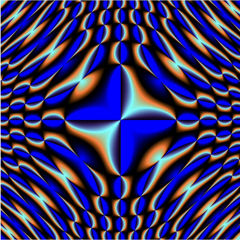
But at large scale it looks like this (the bounding box is approximately -75,000 to 75,000):
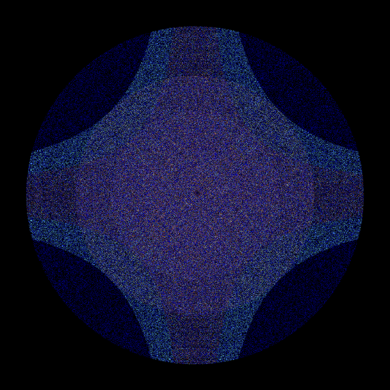
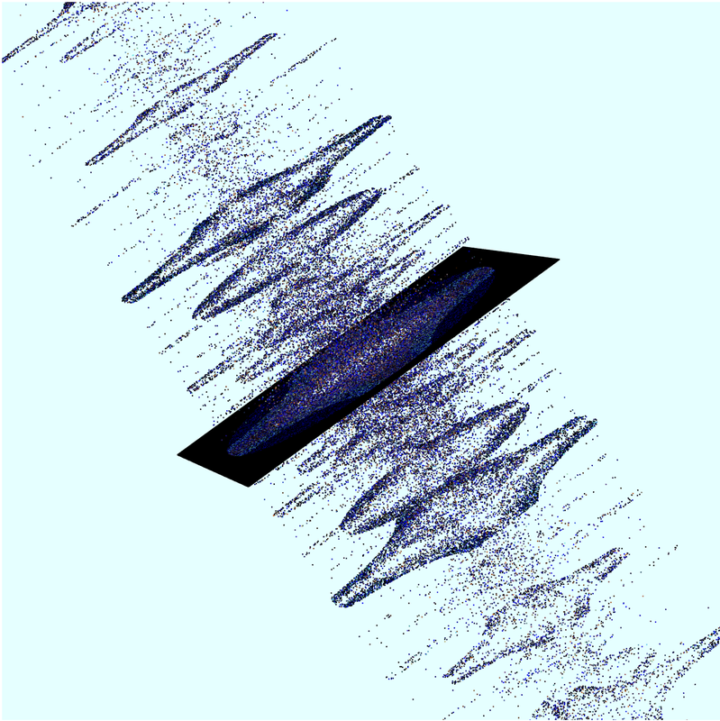
It gets even more interesting when plotted in 3D with normalization turned off and points mode on. When we rotate the plot, we see what appear to be regular layers of points that have roughly equal values:
Helper Functions:
The utility of the function plotter is greatly expanded by the ability to define custom functions which can be called by the expression evaluator.
Functions which do not have a closed form or are otherwise best suited to iterative (or approximate) evaluation can be plotted by defining a helper function and calling it in the expression editor.
An excellent example of a function which does not have a closed form is the Mandelbrot Set
The Mandelbrot Set is defined as the
set of points Z which satisfy the condition that the expression
 is bounded, for all points in the complex plane. To actually know
if a point is in the set or not, we would have to do an infinite number of iterations
for every point!
is bounded, for all points in the complex plane. To actually know
if a point is in the set or not, we would have to do an infinite number of iterations
for every point!
Since that is not possible, the best we can do is do a finite number of
iterations and if a complex number c = x + iy makes
less than some finite bound (4 turns out to be a suitable bound) we declare it to
be in the set.
If we interpret pixel locations on the canvas to be points in the complex plane we can plot an approximation of the Mandelbrot Set. Furthermore, if we color each pixel based on the number of iterations it took to exclude it from the set, a very interesting image is generated–especially if we zoom in on parts of the image.
Here is some code to put into the helper function code editor to render the Mandelbrot:
const float max = 100.0;
float mandelbrot(float fx, float fy) {
  float iteration  = 0.0;
  float x          = 0.0;
  float y          = 0.0;
  float xtemp      = 0.0;

  for ( float i = 0.0; i < max; ++i  )
  {
    if ( sqrt(x * x + y * y) <= 4.0 ) {
      xtemp = x * x - y * y + fx;
      y = 2.0 * x * y + fy;
      x = xtemp;
      iteration = i;
    }
    else{ break; }
  }
  return iteration;
}
We will also need to modify the color function a little:
vec4 getcolor(float z)
{
if (z == max - 1.0) return vec4(0,0,0,1);
z/=max;
float r = z + z > 1.0 ? 1.0 / (z + z) : z + z;
float g = z > 1.0 ? 1.0 / (z * z) : z;
float b = z > 1.0 ? 1.0 / z : z * z;
return vec4(r, g, b, 1.0);
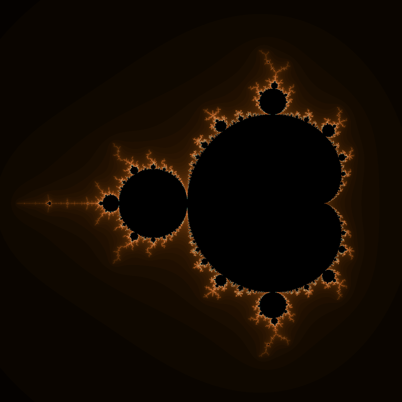
}Now just enter mandelbrot(x, y) in the expression evaluator and click the
Render2D button.
Here is the rendering of the set that you get:
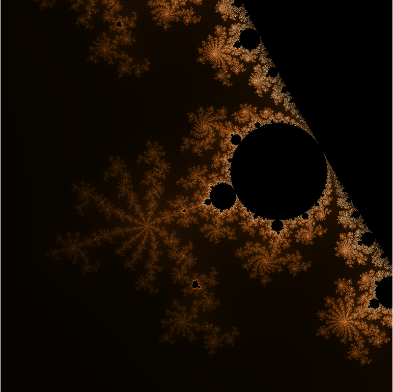
If we zoom in a bit on one of the interior edges and change max to 700.0 we
can see some nice detail:
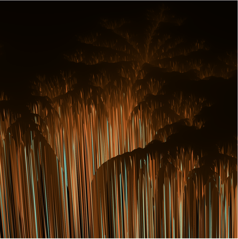
If we transition to 3D mode and tilt the plot a bit we can see the rate at which points were eliminated from the set by their elevation:
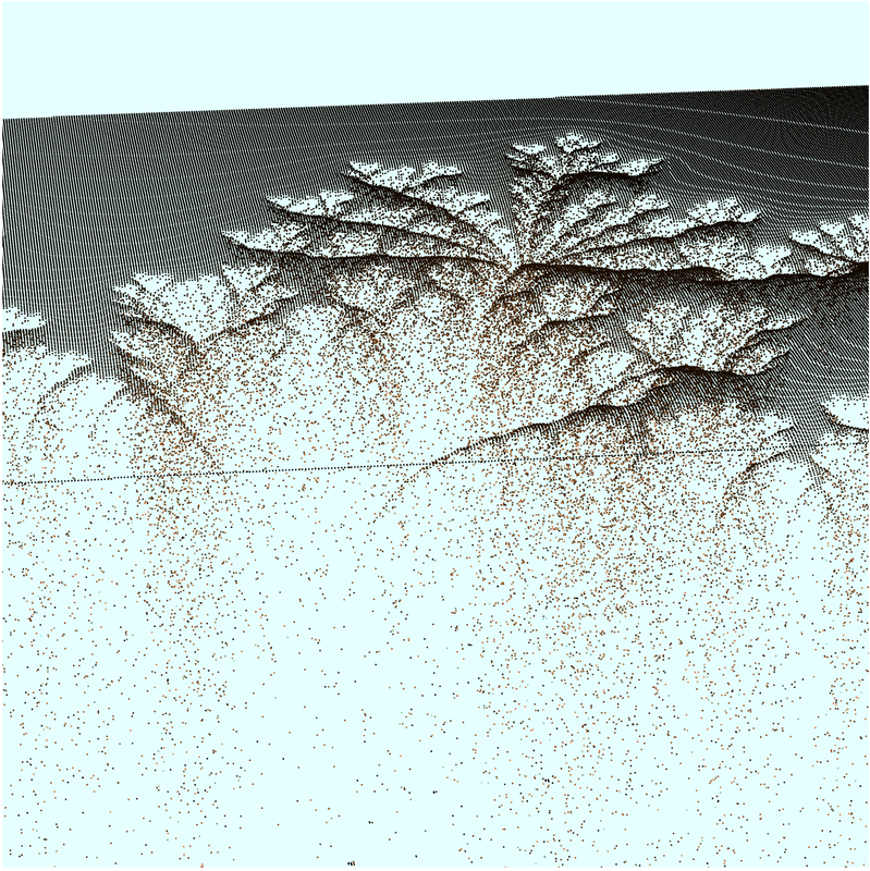
This effect can perhaps more easily be seen if we switch to points mode:
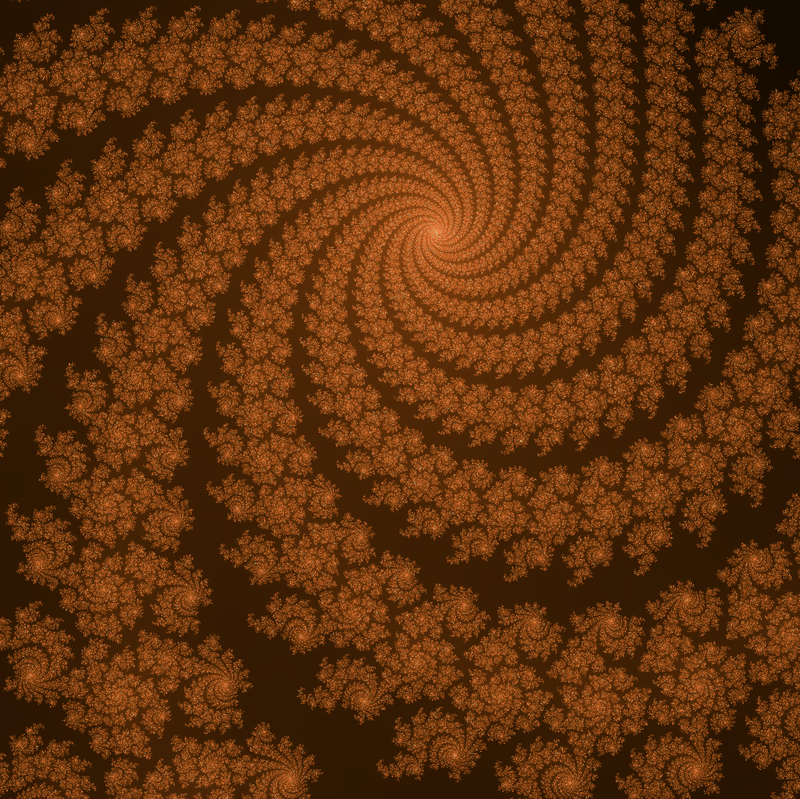
Another example of an interesting non-closed form function is the Julia Set which is similar to the Mandelbrot Set. If we use this code in the helper function editor:
const float max = 100.0;
float julia( float x, float y ) {
  float cRe = -0.7;
  float cIm = 0.27015;
  float z = 0.0;
  float xtemp;
  for(float i = 0.0; i < max; i++)
  {
    xtemp = x * x - y * y + cRe;
    y = 2.0 * x * y + cIm;
    x = xtemp;
    if((x * x + y * y) > 4.0) break;
    z = i;
  }
  return z;
}
we get this rendering (using the same getcolor() function and entering
julia(x, y) in the expression editor):
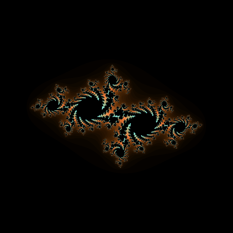
Zooming in and bumping up max to 2000.0 we get:
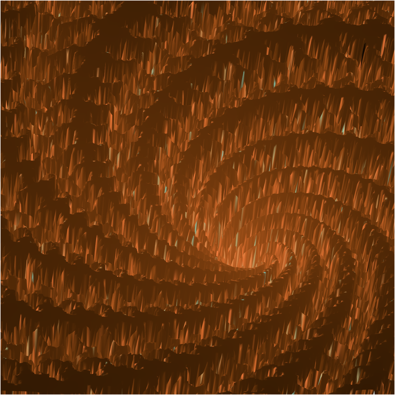
Going 3D (with some rotations and zooming):
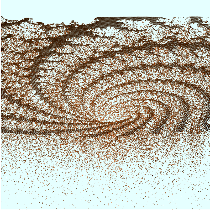
In points mode:
Feel free to contact me with questions/issues at stharding at gmail dot com