| Dennis L. Chao
Department of Computer Science University of New Mexico Albuquerque, NM 87131 U.S.A. Email: dlchao@cs.unm.edu | Miles P. Davenport
Centre for Vascular Research Department of Pathology University of New South Wales Kensington, NSW 2052 Australia Email: m.davenport@unsw.edu.au | Stephanie Forrest
Department of Computer Science University of New Mexico Albuquerque, NM 87131 U.S.A. Email: forrest@cs.unm.edu | Alan S. Perelson
Theoretical Biology and Biophysics Los Alamos National Laboratory Los Alamos, NM 87545 U.S.A. Email: asp@t10.lanl.gov |
Abstract:
We have constructed a computer model of the cytotoxic T lymphocyte (CTL) response to antigen and the maintenance of immunological memory. Because immune responses often begin with small numbers of cells and there is great variation among individual immune systems, we have chosen to implement a stochastic model that captures the life cycle of T cells more faithfully than deterministic models. Past models of the immune response have been differential equation based, which do not capture stochastic effects, or agent-based, which are computationally expensive. We use a stochastic stage-structured approach that has many of the advantages of agent-based modeling but is much more efficient. Our model can provide insights into the effect infections have on the CTL repertoire and the response to subsequent infections.
Collaborations between biologists and computer scientists have produced spectacular results, most notably the sequencing of the human genome. Despite the successes of this collaboration, most current approaches are a long way from allowing us to model complex biological systems, much less entire organisms. We believe that computer scientists can play a more integrated role in their collaboration with biologists than simply applying existing algorithms from computer science, or inventing new ones, to data from molecular biology. Computer modeling provides an alternative to the animal models traditionally used by biologists, and it complements the capabilities of deterministic mathematical models. Computer modeling allows one to integrate a wealth of experimental findings into a coherent system that can provide great insight into biological systems.
Based on a variety of experimental results from the literature, we have constructed a computer model of a major component of the mammalian immune system, the cytotoxic T lymphocyte (CTL) response. Our ultimate goal is to use the model to provide insight into the pathology and possible treatments of diseases such as AIDS, flu, cancer, and autoimmune disorders. In the process of building the model we were able to situate experimental data from multiple experiments in a coherent framework that forms a relatively complete and consistent interpretation of T cell behavior. We take a computationally efficient stage-structured modeling approach which allows us to incorporate available biological data relatively easily, resulting in a model that makes quantitative predictions. In the sections that follow, we briefly review the CTL response to infections, discuss other approaches to modeling the immune system, describe our own model of CTL responses, and illustrate its behavior in three different settings.
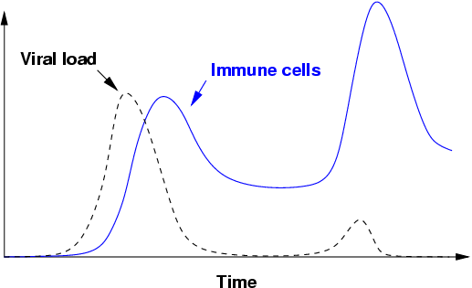
CTLs play a unique role in our immune systems. They reside in tissue or circulate through the body via the blood and lymph to detect cells that have been compromised by foreign organisms, such as viruses and bacteria. After the first exposure to a virus, T cells rapidly replicate and attack infected cells in a primary response. The T cell population then decreases, leaving behind a population of long-lived memory cells (Figure 1). The virus is typically eliminated within two weeks. If the individual is infected again by the same virus, the memory T cells mount a much larger and faster secondary response, which can often clear an infection before it becomes symptomatic. Thus, each infection prepares the immune system to be more effective in subsequent encounters. However, this response is very specific to a particular infectious agent and will usually not protect the individual from unrelated viruses. A lifetime of exposure to pathogens shapes an organism's repertoire of memory cells, making the states of different individuals' immune systems unique.
Figure 1: A schematic representation of the primary and secondary T cell responses to infection. A virus enters the body and rapidly infects the host (dotted line). The cells of the immune system (solid line) respond by replicating and eliminating the virus. Upon a second exposure to the same virus, the immune system eliminates the virus before massive infection occurs.
The above description is a population-level view of the immune response. The behaviors of the virus and T cell populations are described in the aggregate, not as the actions of individual cells. T cells have traditionally been studied using functional assays, in which the behavior of a culture of cells is studied in vitro. These kinds of data give information about the behavior of populations of cells. Newer technologies, such as CFSE labeling [27] and two-photon laser microscopy [9], allow immunologists to observe or infer the behavior of T cells at the level of the individual cell in vivo. These newer data provide a different view of immune cell behavior that must be reconciled with earlier population-level results. We claim that stochastic modeling techniques, described in the next section, will allow us to integrate these two kinds of data.
Differential equation models have long been used for immune system modeling [4,14,38,37,20,32,6,1]. In these models, populations of antigens and immune cell types are continuous variables in systems of ordinary differential equations (ODEs). Analytical techniques allow modelers to define regimes of system behavior and their associated parameters and initial conditions. For example, one can determine the model parameters for which an infection is effectively cleared by the immune system [6]. The solutions capture the average behavior of large populations of perfectly mixed, identical cells. Many techniques that could make these models more faithful to biological reality, such as adding time delays or partial differential equations [1], complicate solving the models analytically or even numerically. Moreover, data on the behavior of individual cells is difficult to incorporate directly, and these data must generally be recast as population-level phenomena. For example, we can estimate both the minimum and average time it takes for a cell to divide, but an ODE model would typically express population growth using only the average cell cycle time.
Agent-based simulation is a promising new technique made feasible with the advent of greater computer power. These systems monitor the actions of a large number of simple entities, or agents, in order to observe their global behavior. Each agent consists of state variables and a set of rules that governs its behavior, and they can interact either directly with each other or indirectly through the environment. Because all individuals in a population are explicitly represented, they can have unique histories and behaviors. The global behavior of these agents is observed in a discrete time or event-driven simulation.
Agent-based modeling has many features suited to modeling the immune response. It is adept at incorporating stochastic events, which appear to be crucial in regulating immune function [17]. A single chance event, such as the serendipitous recognition of a cancer antigen by a single cell in the immune system, can determine the fate of an organism [33]. The addition of randomness to a model allows one to explore the distribution of possible outcomes, as in [13], as opposed to only the single most likely one addressed by most mathematical models. This is especially valuable when studying immune responses, as even genetically identical individuals can exhibit different responses to the same antigen [26]. Because small numbers of cells are involved at the beginning of an immune response [16,7], using a discrete model might be more suitable than a continuous one. The existing agent-based models of the immune system, such as IMMSIM [10,39,23], the B cell model of Smith et al. [41], and the self-nonself discrimination model of Langman and Cohn [11,24], take advantage of these features. Another advantage of agent-based models is that by explicitly representing the individual cells, they are in many ways closer to the modeled system. In contrast to population-level models, agent-based model parameters correspond to actual properties of the cells, and the output of these models can be processed so that they can be observed at the any level, from the level of the individual cells to the population level.
Unfortunately, agent-based modeling can be computationally costly. The CTL population alone may have as many as 1012 cells in a human, and running a model with this many distinct entities would be prohibitive. To address such problems, agent-based models can be implemented to take advantage of multiple computers, such as the parallel version of IMMSIM known as PARIMM[5]. Because agent-based models must be run many times to characterize the distribution of outcomes, they should be as simple and efficient as possible without sacrificing essential aspects of the immune response. Using techniques such as lazy evaluation [40] allows models to instantiate only cells that participate in an immune response, but a response in a mouse can involve on the order of CTLs [8], which is still a large number to simulate explicitly.
For computational efficiency, we have chosen to use a stochastic stage-structured approach [28] to modeling the immune response. Stage-structured models have long been used to model populations in ecology [25,43] but have not yet been applied to immune systems. In these models, an individual's life cycle is divided into stages, such as developmental maturity or body size. All individuals in a given stage are assumed to be identical. Therefore, only a single integer is required to represent the individuals in a given stage, rather than the data structure per individual needed by an agent-based approach. By making our model orders of magnitude more efficient than equivalent agent-based models, we can easily run the model a larger number of times and on less powerful computers. The transition probabilities between these stages is specified, and the model can be used to predict the demographics of a given initial population over time. Stochasticity can be added to the model if needed, for example to model the distribution of possible outcomes. Analytical techniques have been developed for these models, but when there are interacting populations, in our case T cells, infected cells, and virus, it is easier to run the model on a computer multiple times. In order to allow T cells to interact with the viral infection, we run the T cell model and the viral model synchronously and at each time step the populations can interact. For example, at some stages T cells can eliminate infected cells, so at each time step the number of infected cells is reduced by a function of the number of T cells that are in these stages.
By using discrete rather than continuous populations and by explicitly specifying the actions and transitions of cells as probabilities per individual cell, our model enforces the realistic behavior of individual cells without the computational cost of representing each cell explicitly. We strike a balance between the unrealistically small number of populations used by analytical approaches and the unwieldy one-agent-per-cell implementations of agent-based models. Because we do not intend to solve our system analytically, we can accommodate multiple cell states. However, to make the model more efficient than an equivalent agent-based model, we must limit the number of possible cell states to a manageable number (described in section 5).
We can infer much of the life cycle of CTLs at the cellular level from experimental data. For simplicity, the description that follows omits many essential components of the immune response, such as the innate immune system, dendritic cells, and CD4 T cells; their role in facilitating the CTL response is implicit in the model.
T cell precursors are generated in the bone marrow and mature in the thymus. Each T cell responds to a particular peptide bound in the groove of a particular cell surface protein, called a major histocompatibility (MHC) molecule. The total repertoire of T cells covers an enormous range of possible MHC-peptide complexes. As a consequence, there is the possibility that some of these T cells will react to the body's own cells. The thymus performs selection on these new T cells, only allowing those that are not likely to react to the body to mature and leave the thymus. Once mature, T cells migrate to secondary lymphoid organs where they essentially lie dormant as naïve cells. When a naïve cell is exposed to its cognate peptide in sufficient quantity, it is committed to a programmed response that causes it to divide and become an effector cell even in the absence of further antigenic stimulation [21,44]. Larger doses of antigen can induce larger responses primarily by stimulating a greater number of naïve cells, not by stimulating individual cells to a larger degree [21]. For the first 24 hours, the newly activated T cells do not replicate [34,18,45,44], but after this initial phase, they can rapidly divide a fixed number of times and acquire effector functions, such as cytotoxicity (i.e., the ability to kill cells) [21]. Effector CTLs kill cells either by releasing perforins that create holes in the target cell's membrane or by triggering apoptosis, or cell suicide, in the target. During this period of rapid expansion, the cells also have a high death rate, reducing net population growth. After the programmed division cycles, the death rate dominates CTL kinetics and the population declines rapidly [3]. If the pathogen is not cleared by this time, the remaining T cells might stop responding to infected cells.
Although most of the T cells participating in the response die, a small subpopulation persists as memory cells [30]. Memory cells are able to mount a faster and more aggressive secondary response in future encounters with the same or closely related pathogens [15]. Upon antigenic stimulation, memory cells begin to proliferate almost immediately and develop cytotoxicity within a few hours [2]. Their replication rates are approximately the same as effectors in the primary response, but their lower death rates allow them to accumulate faster [45,19]. In addition, both the shorter time to acquire effector functions and the larger starting populations allow them to clear infected cells much faster than effectors in the primary response can. Immunological memory forms the basis of vaccination, in which an organism is exposed to viral antigens in order to build immune memory to the virus.
Figure 2: A simplified state transition diagram for the T cell life cycle. The actual model has hundreds of states.
We have incorporated the elements of the T cell life cycle into a model. The number of possible T cell states in our model is in the hundreds, but because T cells basically follow a linear development path [35], the number of state transition probabilities we need to define is small (Figure 2). In fact, most of these states are needed solely to keep track of the amount of time a cell needs to wait before it can transition between two other states, so most of the transition probabilities are 1.
Our model runs in discrete one-hour time steps, and all entities in the model act synchronously at each time step. If it takes 24 hours for a cell to transition from state to state , 24 separate stages would represent the cells that are in the process of this transition, one for each hour. At the end of each simulation hour, the members of each of these stages are automatically promoted to the next. Using a smaller time step would require the model to have more states, while a larger step would yield less accurate results. Many transitions in the model are stochastic, and instead of automatically transferring all members of a stage, only a random fraction of them are. In such situations, we assume that all members of a stage have the same probability of transitioning, and the number that transition in a given hour could be determined by generating random values between 0 and 1 then counting the number that are less than . For computational efficiency, rather than generating random values we generate only one uniformly distributed random value and use it to draw from a binomial distribution , which gives the same overall behavior.
Naïve T cells specific to a particular antigen are in the same stage until they are stimulated. Our model accommodates T cells of different specificities by instantiating separate stage-based models for each, but for the purposes of discussion we will assume that there is only one T cell specificity. As naïve cells are stimulated, they are promoted through a series of 19 stages that represent the 19 hours before a naïve cell can begin its programmed response. The cells in these stages do not interact with infected cells, but when they emerge after 19 simulation hours, they become effectors and start responding to infected cells and dividing. In our model, T cells take a minimum of 5 hours to divide, so the first T cell divisions can take place 24 hours after antigenic stimulation, which agrees with experimental findings.
Infected cells, uninfected cells, and virus levels are modeled by a set of difference equations that interact with the T cell models at each time step. In this model of viral infection, viruses infect uninfected cells, converting them to infected cells, which in turn produce more virus [46,36,31]. A constant source replenishes the pool of uninfected cells, which allows the body to recover after infection. We use deterministic difference equations because the number of infected cells is generally large, so using a random number generator to add stochasticity would have little effect.
We implement the programmed divisions of effector cells by keeping track of the number of times a cell divides. Each new effector cell is placed in a stage of effectors that have not yet divided. When one reproduces, it is moved with its daughter to the next division stage. After 15 divisions (about 5 days of replicating), the cells stop dividing [3]. Therefore, the model simply needs to store values for the number of cells that have divided 0 through 15 times, which is much more efficient than storing the ages of billions of individual effector cells. After the cells stop dividing at the end of the programmed response, the high death rate in effect during the entire response causes the cell population to rapidly decline.
A cell can not divide arbitrarily quickly, and we enforce a minimum division time by using a 2-phase cell cycle model [42]. A cell cycle starts in A phase , during which the cell does not divide. At each time step, a cell has a constant probability of entering phase B, which has a fixed length. At the end of the B phase, both the parent cell and the new daughter cell enter the A phase of the next division stage. Therefore, a cell's minimum time to division is the length of the B phase. Without this phase, some cells could divide an arbitrarily large number of times in a time interval.
To implement the 2-phase cell cycle model, each division stage is further divided into sub-stages in the A phase and B phase. At each time step we draw from a binomial distribution to determine the number of cells in the A sub-stage that transition to B. We also allocate one sub-stage per time step that the cells remain in B phase, and cells in these sub-stages are promoted to the next stage at each simulated hour. We use one-hour time steps, so if cells remain in B phase for n hours, there will be n B phase sub-stages per division stage. We assume that the minimum time to division is about 5 hours [44], so each division stage's B phase has 5 sub-stages. If we assume that a T cell can divide 50 times, there could to be up to 300 subpopulations of cells per T cell clone, or 50 A phase subpopulations and 250 B phase subpopulations. These 300 subpopulations efficiently represent the millions of effectors that can originate from a single T cell clone in an immune response.
After 5 cell divisions [34,35], effector cells have a constant probability per time step of becoming memory cells, which results in a final memory pool that is about 5% of the size of the peak response [12]. It can take 2 or 3 weeks for a cell to develop a full memory cell phenotype after the initial infection [22]. Therefore, memory cells are not likely to join the immune response that initially generated them. Memory cells are dormant until antigenic stimulation. When stimulated by antigen, they can rapidly start responding to the infection.
The current version of this model, written in Java, is available upon request from the first author. We chose to implement the program in Java to make it platform-independent, and we have found its performance to be satisfactory.
Our model reproduces population-level phenomena seen experimentally in laboratory mice, and we describe some of these results below. We begin with an experiment that illustrates the basic differences between primary and secondary responses, then proceed to describe our model of experiments that replicate results found in laboratory experiments.
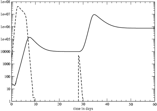
Figure 3: Primary and secondary CTL responses to viral infection. The dashed lines represent virus levels, with the secondary exposure to the virus at day 28. The solid line represents the number of T cells specific to this virus, including naïve, effector, and memory cells.
We simulated the primary and secondary responses to an acute infection (Figure 3). For this trial, we were not attempting to match our results to a particular experiment but were instead interested in testing the overall dynamics of the T cell response in the model. We simulated the injection of 5,000 virus particles into a mouse, and the primary response began after approximately one day. The response peaked at day 7 then declined to form a stable memory pool. At day 28, an identical injection was administered, and the secondary response was faster and larger than the primary. The secondary response began almost immediately after the second exposure to the virus, and the lower death rate of memory-derived effectors [19] caused the T cell population to increase more rapidly than in the primary response. The secondary response also generated a larger pool of stable memory cells. Therefore, the simulated mouse's immunological memory could be ``boosted'' by multiple exposures to the same antigen, making future responses to it even more effective.
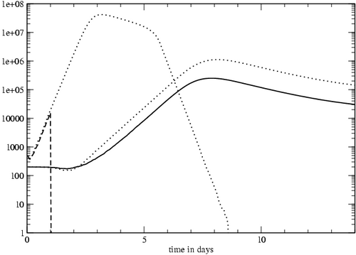
One of the implications of the programmed T cell response is that the immune response is initiated by antigen but its outcome is antigen-independent. If this is the case, then removing antigen after the start of a response should not affect it. This was tested in mice infected by the bacterium L. monocytogenes [29,3]. Antibiotics were administered to eliminate the bacteria 24 hours after inoculation, which quickly removed all antigen. The peak of the T cell response occurred at the same time in the mice administered antibiotics and in the control mice, which were not given antibiotics. The early elimination of infected cells only caused a small reduction in the magnitude of the responses. The removal of antigen did not greatly affect the timing or the magnitude of the T cell response.
Our model predicts a similar outcome (Figure 4). The reduced response in our model was due to the shortened recruitment time for naïve cells; when the simulated infection was eliminated after 36 hours instead of 24, the magnitude of the T cell response matched that of the control case (data not shown). Incorporating the programmed response might be essential to modeling the efficacy of vaccinations. Vaccines often use attenuated strains of pathogens that have diminished reproductive capacity and are rapidly cleared from the body. If the purpose of a vaccine is to induce a large response in order to build a large pool of specific memory cells, then a large dose of an attenuated virus might be effective even if the virus level drops rapidly. If the T cell response were totally antigen-dependent, short periods of antigenic stimulation would not initiate an adequate response.
Figure 4: T cell response to an infection interrupted by antibiotic treatment. The antigen (dashed line) was removed from the system after 24 hours. The T cell response (solid line) is almost unaffected by the removal of antigen. The antigen and T cell levels of the control case, in which the antigen is not removed, are plotted for comparison (dotted lines).
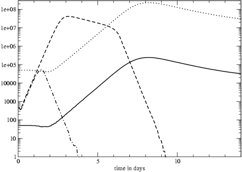
Figure 5: The effect of increasing the number of naïve cells. One model run started with 50 naïve cells (solid line) and a modest virus load (dashed line). The other model run started with 50,000 naïve cells (dotted line) and the same virus load (dash-dot line).
The size of the initial naïve cell population can affect the outcome of an infection. Presumably, increasing the number of naïve cells can result in a larger and more effective response to infection. This hypothesis was tested experimentally in mice [16]. The number of naïve cells in mice was experimentally increased before infection in order to determine how the number of responding naïve cells affects the T cell response to an acute infection. Increasing the number of naïve cells by 1000-fold moved the peak of the infection between 1 and 2 days earlier and reduced the viral load by about 2 logs. In other words, the infection was smaller and eliminated sooner. Our model's results are in agreement with the mouse experiments; increasing the number of naïve cells in the model 1000-fold, the peak virus load was one day earlier and between 2 and 3 logs smaller than in the control case (Figure 5).
We have presented a model of the CTL response and memory formation that features realistic behavior at the level of the individual cells yet is more efficient than standard agent-based approaches to modeling. In doing so, we are able to incorporate various stages of the T cell life cycle using the most detailed observations from laboratory experiments. The model yields results that are consistent with experiment.
The value of modeling goes beyond simply predicting the behavior of a system. The process of building the model highlights gaps and inconsistencies in our understanding of the immune response. If our model produces unrealistic results, then we can modify and test the assumptions made on the immune-cell level to rectify the model's output. The most plausible of these models can become working hypotheses of T cell behavior that experimentalists could verify in the lab. The creation of models tests the intuition of immunologists. When the mechanisms of the immune response are studied in reductionistic detail, it is easy to lose sight of the system as a whole. Our model integrates the knowledge gained in laboratory experiments to form a coherent system that simulates an immune response. Our preliminary results show that the model can reproduce a wide variety of laboratory results. This approach to bridging the gap between cellular-level and whole organism studies requires close collaborations between experimental biologists and computer scientists.
This work was supported by the National Science Foundation (ANIR-9986555), the Office of Naval Research (N00014-99-1-0417), the Defense Advanced Research Projects Agency (AGR F30602-00-2-0584), the National Institutes of Health (NIH R37 AI28433), the James S. McDonnell Foundation (21st Century Research Awards / Studying Complex Systems), the Intel Corporation, and the Santa Fe Institute. Portions of this work were done under the auspices of the US Department of Energy and supported under contract W-7405-ENG-36.
This document was generated using the LaTeX2HTML translator Version 2K.1beta (1.48)
Copyright © 1993, 1994, 1995, 1996,
Nikos Drakos,
Computer Based Learning Unit, University of Leeds.
Copyright © 1997, 1998, 1999,
Ross Moore,
Mathematics Department, Macquarie University, Sydney.
The command line arguments were:
latex2html -dir html -split 0 ieee.tex
The translation was initiated by Dennis Chao on 2003-06-09
The output from latex2html was then hand-edited by Dennis Chao.